Computational grids and boundary / initial / first guess conditions

The computational spatial grid must be defined by the user. The orientation (direction) can be chosen arbitrarily.


The boundaries of the computational spatial grid in SWAN are either land or water. In the case of land there is no problem: the land does not generate waves and in SWAN it absorbs all incoming wave energy. But in the case of a water boundary there may be a problem. Often no wave conditions are known along such a boundary and SWAN then assumes that no waves enter the area and that waves can leave the area freely. These assumptions obviously contain errors which propagate into the model. These boundaries must therefore be chosen sufficiently far away from the area where reliable computations are needed so that they do not affect the computational results there. This is best established by varying the location of these boundaries and inspect the effect on the results. Sometimes the waves at these boundaries can be estimated with a certain degree of reliability. This is the case if (a) results of another model run are available (nested computations) or, (b) observations are available. If model results are available along the boundaries of the computational spatial grid, they are usually from a coarser resolution than the computational spatial grid under consideration. This implies that this coarseness of the boundary propagates into the computational grid. The problem is therefore essentially the same as if no waves are assumed along the boundary except that now the error may be more acceptable (or the boundaries are permitted to be closer to the area of interest). If observations are available, they can be used as input at the boundaries. However, this usually covers only part of the boundaries so that the rest of the boundaries suffer from the same error as above.


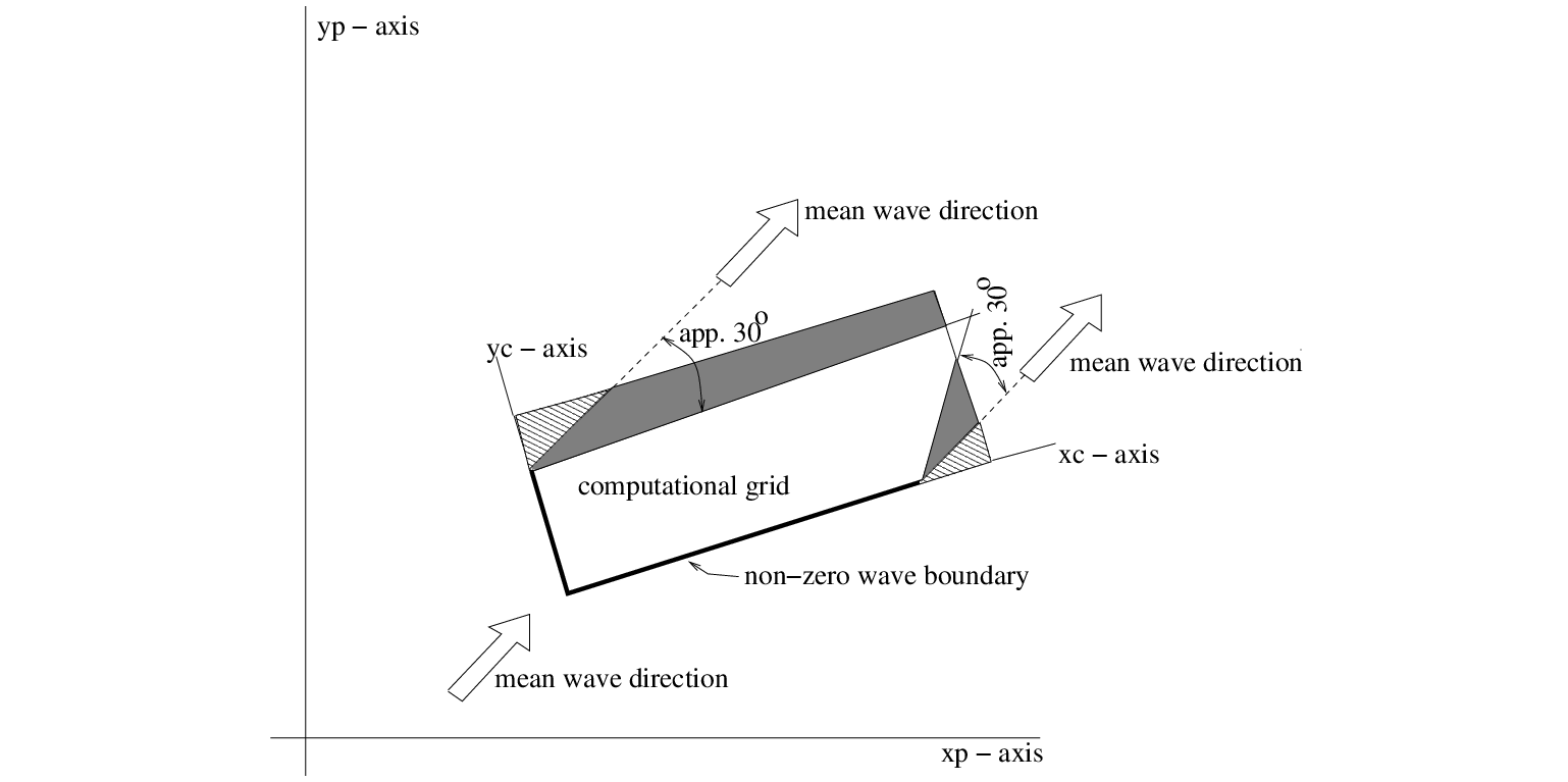
A special case occurs near the coast. Here it is often possible to identify an up-wave boundary (with proper wave information) and two lateral boundaries (with no or partial wave information). The affected areas with errors are typically regions with the apex at the corners of the water boundary with wave information, spreading towards shore at an angle of 30$^{{\rm o}}$ to 45$^{{\rm o}}$ for wind sea conditions to either side of the imposed mean wave direction (less for swell conditions; the angle is essentially the one-sided width of the directional distribution of wave energy). For propagation of short crested waves (wind sea condtions) an example is given in Figure 2.1. For this reason the lateral boundaries should be sufficiently far away from the area of interest to avoid the propagation of this error into this area. Such problems do not occur if the lateral boundaries contain proper wave information over their entire length e.g. obtained from a previous SWAN computation or if the lateral boundaries are coast.

Figure 2.1: Disturbed regions in the computational grid due to erroneous boundary conditions are indicated with shaded areas.

When output is requested along a boundary of the computational grid, it may occur that this output differs from the boundary conditions that are imposed by the user. The reason is that SWAN accepts only the user-imposed incoming wave components and that it replaces the user-imposed outgoing wave components with computed outgoing components (propagating to the boundary from the interior region). The user is informed by means of a warning in the output when the computed significant wave height differs more than 10%, say (10% is default), from the user-imposed significant wave height (command BOUND...). The actual value of this difference can be set by the user (see the SET command). Note that this warning will not apply in the case of unstructured grids.


If the computational grid extends outside the input grid, the reader is referred to Section 2.6.2 to find the assumptions of SWAN on depth, current, water level, wind, bottom friction, vegetation, mud, and ice in the non-overlapping area.


The spatial resolution of the computational grid should be sufficient to resolve relevant details of the wave field. Usually a good choice is to take the resolution of the computational grid approximately equal to that of the bottom or current grid. If necessary, an unstructured grid may be used.


SWAN may not use the entire user-provided computational grid if the user defines exception values on the depth grid (see command INPGRID BOTTOM) or on the curvilinear computational grid (see command CGRID). A computational grid point is either

• wet, i.e. the grid point is included in the computations since it represents water; this may vary with time-dependent or wave-induced water levels or
• dry, i.e. the grid point is excluded from the computations since it represents land which may vary with time-dependent or wave-induced water levels or
• exceptional, i.e. the grid point is permanently excluded from the computations since it is so defined by the user.

If exceptional grid points occur in the computational grid, then SWAN filters the entire computational grid as follows:

• each grid line between two adjacent wet computational grid points (a wet link) without an adjacent, parallel wet link, is removed,
• each wet computational grid point that is linked to only one other wet computational grid point, is removed and
• each wet computational grid point that has no wet links is removed.

The effect of this filter is that if exception values are used for the depth grid or the curvilinear computational grid, one-dimensional water features are ignored in the SWAN computations (results at these locations with a width of about one grid step may be unrealistic). If no exception values are used, the above described filter will not be applied. As a consequence, one-dimensional features may appear or disappear due to changing water levels (flooding may create them, drying may reduce two-dimensional features to one-dimensional features).


It must be noted that for parallel runs using MPI the user must indicate an exception value when reading the bottom levels (by means of command INPGRID BOTTOM EXCEPTION), if appropriate, in order to obtain good load balancing.


The computational time window must be defined by the user in case of nonstationary runs. The computational window in time must start at a time that is early enough that the initial state of SWAN has propagated through the computational area before reliable output of SWAN is expected. Before this time the output may not be reliable since usually the initial state is not known and only either no waves or some very young sea state is assumed for the initial state. This is very often erroneous and this erroneous initial state is propagated into the computational area.


The computational time step must be given by the user in case of nonstationary runs. Since, SWAN is based on implicit numerical schemes, it is not limited by the Courant stability criterion (which couples time and space steps). In this sense, the time step in SWAN is not restricted. However, the accuracy of the results of SWAN are obviously affected by the time step. Generally, the time step in SWAN should be small enough to resolve the time variations of computed wave field itself. Usually, it is enough to consider the time variations of the driving fields (wind, currents, water depth, wave boundary conditions). But be careful: relatively(!) small time variations in depth (e.g. by tide) can result in relatively(!) large variations in the wave field.


As default, the first guess conditions of a stationary run of SWAN are determined with the 2$^{{\rm nd}}$ generation mode of SWAN. The initial condition of a nonstationary run of SWAN is by default a JONSWAP spectrum with a $\cos ^{2} (\theta )$ directional distribution centred around the local wind direction.


A quasi-stationary approach can be employed with stationary SWAN computations in a time-varying sequence of stationary conditions.


The computational spectral grid needs to be provided by the user. In frequency space, it is simply defined by a minimum and a maximum frequency and the frequency resolution which is proportional to the frequency itself (i.e. logarithmic, e.g., $\Delta\, f\,\, =\,\, 0.1\,\, f$). The frequency domain may be specified as follows (see command CGRID):

• The lowest frequency, the highest frequency and the number of frequencies can be chosen.
• Only the lowest frequency and the number of frequencies can be chosen. The highest frequency will be computed by SWAN such that $\Delta\, f\,\, =\,\, 0.1\,\, f$. This resolution is required by the DIA method for the approximation of nonlinear 4-wave interactions (the so-called quadruplets).
• Only the highest frequency and the number of frequencies can be chosen. The lowest frequency will be computed by SWAN such that $\Delta\, f\,\, =\,\, 0.1\,\, f$. This resolution is required by the DIA method for the approximation of nonlinear 4-wave interactions.
• Only the lowest frequency and the highest frequency can be chosen. The number of frequencies will be computed by SWAN such that $\Delta\, f\,\, =\,\, 0.1\,\, f$. This resolution is required by the DIA method for the approximation of nonlinear 4-wave interactions.

The value of lowest frequency must be somewhat smaller than 0.7 times the value of the lowest peak frequency expected. The value of highest frequency must be at least 2.5 to 3 times the highest peak frequency expected. For the XNL approach, however, this should be 6 times the highest peak frequency. Usually, it is chosen less than or equal to 1 Hz.


SWAN has the option to make computations that can be nested in WAM or WAVEWATCH III. In such runs SWAN interpolates the spectral grid of WAM or WAVEWATCH III to the (user provided) spectral grid of SWAN. The WAM Cycle 4 source term in SWAN has been retuned for a highest prognostic frequency (that is explicitly computed by SWAN) of 1 Hz. It is therefore recommended that for cases where wind generation is important and WAM Cycle 4 formulations are chosen, the highest prognostic frequency is about 1 Hz.


In directional space, the directional range is the full 360$^{{\rm o}}$ unless the user specifies a limited directional range. This may be convenient (less computer time and/or memory space), for example, when waves travel towards a coast within a limited sector of 180$^{{\rm o}}$. The directional resolution is determined by the number of discrete directions that is provided by the user. For wind seas with a directional spreading of typically 30$^{{\rm o}}$ on either side of the mean wave direction, a resolution of 10$^{{\rm o}}$ seems enough whereas for swell with a directional spreading of less than 10$^{{\rm o}}$, a resolution of 2$^{{\rm o}}$ or less may be required. If the user is confident that no energy will occur outside a certain directional sector (or is willing to ignore this amount of energy), then the computations by SWAN can be limited to the directional sector that does contain energy. This may often be the case of waves propagating to shore within a sector of 180$^{{\rm o}}$ around some mean wave direction.


It is recommended to use the following discretization in SWAN for applications in coastal areas:

direction resolution for wind sea	$\Delta \theta = 15^o - 10^o$
direction resolution for swell	$\Delta \theta = 5^o - 2^o$
frequency range	$0.04 \leq f \leq 1.00$ Hz
spatial resolution	$\Delta x, \Delta y = 50 - 1000$ m

The numerical schemes in the SWAN model require a minimum number of discrete grid points in each spatial directions of 2. The minimum number of directional bins is 3 per directional quadrant and the minimum number of frequencies should be 4.


A final remark on the choice of spatial and spectral resolution. SWAN should not shift energy more than one spectral bin ($\Delta f$ and/or $\Delta \theta$) when propagating over one spatial grid cell ($\Delta x$ and/or $\Delta y$). This is for reasons for accuracy and not stability. See for details Section 3.8 of the Scientific/Technical documentation. This implies that although SWAN will be stable, whatever resolution you choose, you need to balance spectral and spatial resolution. This could mean, i.e. not necessarily, that you have to refine your spatial resolution when you refine your spectral resolution.


In a situation with currents this is particularly important at the highest frequencies where the Doppler shifts are largest. However, it may well be that inaccuracies thus generated will be removed by the source terms. In other words, accurate Doppler shifts at high frequencies require high spectral and spatial resolution, but the effects may be dominated by white capping. Hence, at the high frequencies, the problem is perhaps masked by white capping. The inaccuracies may only appear at the lowest frequencies, where usually the source terms are relatively weak at these frequencies.


Another issue concerns the excessive wave turning of relatively long waves at shallow water, or cases with depth varies considerably over one spatial grid step, e.g. at the edge of shelf break or seamount at deep ocean. As the refraction becomes excessive in a region with steep bottom gradients, it is possible that the wave energy focus toward a single grid point, creating unrealistically large wave heights and long periods; see Dietrich et al. (2013).


SWAN can optionally uses a Courant-type limiter (see command NUMERIC). This limiter is locally in geographic space for cosmetic reasons, but it avoids propagating a large error to the rest of the geographic domain and thus improve the solution there. However, if the limiter is activated, the computation is still inaccurate, but less so as you are farther from the location with poor resolution. The common mistake people often make is that the limiter may affect the model results negatively, which is, however, not entirely true. As the resolution is too coarse, the model results are inaccurate anyway. Hence, the proper solution to this problem is to choose a suitable resolution, both spectral and spatial, and one can thus avoid the use of the limiter.