Next: Command syntax Up: swanuse Previous: Lock-up Index
In SWAN a number of variables are used in input and output. Most of them are related to waves. The definitions of these variables
are mostly conventional.
| HSIGN | Significant wave height, denoted as  in meters, and defined as in meters, and defined as |
|
 |
||
where
 is the variance density spectrum and is the variance density spectrum and 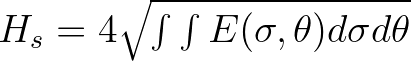 is the absolute is the absolute |
||
| radian frequency determined by the Doppler shifted dispersion relation. | ||
| However, for ease of computation, can be determined as follows: |
||
 |
||
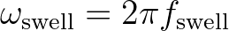
| HSWELL | Significant wave height associated with the low frequency part of | |
the spectrum, denoted as
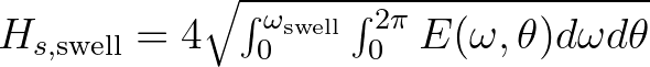 in meters, and defined as in meters, and defined as |
||
 |
||
with
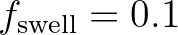 and and
 Hz by default (this can be changed Hz by default (this can be changed |
||
| with the command QUANTITY). | ||
| TMM10 | Mean absolute wave period (in s) of
, defined as |
|
 |
||
| TM01 | Mean absolute wave period (in s) of
, defined as |
|
 |
||
| TM02 | Mean absolute wave period (in s) of
, defined as |
|
 |
||
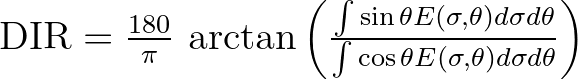
| DIR | Mean wave direction (in  , Cartesian or Nautical convention), , Cartesian or Nautical convention), |
|
| as defined by (see Kuik et al. (1988)): | ||
 |
||
| This direction is the direction normal to the wave crests. | ||
| PDIR | Peak direction of
 |
|
| (in , Cartesian or Nautical convention). |
||
| TDIR | Direction of energy transport (in , Cartesian or Nautical convention). |
|
| Note that if currents are present, TDIR is different from the mean wave | ||
| direction DIR. | ||
| RTMM10 | Mean relative wave period (in s) of
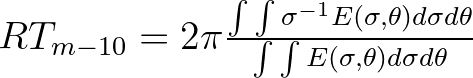 , defined as , defined as |
|
 |
||
| This is equal to TMM10 in the absence of currents. | ||
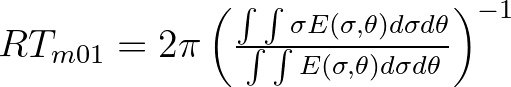
| RTM01 | Mean relative wave period (in s) of
, defined as |
|
 |
||
| This is equal to TM01 in the absence of currents. | ||
| RTP | Relative peak period (in s) of 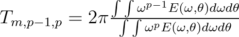 (equal to absolute peak period (equal to absolute peak period |
|
| in the absence of currents). | ||
| Note that this peak period is related to the absolute maximum bin of the | ||
| discrete wave spectrum and hence, might not be the 'real' peak period. | ||
| TPS | Relative peak period (in s) of . |
|
| This value is obtained as the maximum of a parabolic fitting through the | ||
| highest bin and two bins on either side the highest one of the discrete | ||
| wave spectrum. This 'non-discrete' or 'smoothed' value is a better | ||
| estimate of the 'real' peak period compared to the quantity RTP. | ||
| PER | Average absolute period (in s) of
, defined as |
|
 |
||
The power  can be chosen by the user by means of the QUANTITY can be chosen by the user by means of the QUANTITY |
||
command. If  (the default value) PER is identical to TM01 and (the default value) PER is identical to TM01 and |
||
if 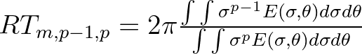 , PER = TMM10. , PER = TMM10. |
||
| RPER | Average relative period (in s), defined as | |
 |
||
| Here, if , RPER=RTM01 and if , RPER=RTMM10. |
||
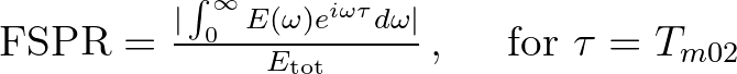
| FSPR | The normalized frequency width of the spectrum (frequency spreading), | |
| as defined by Battjes and Van Vledder (1984): | ||
 |
||
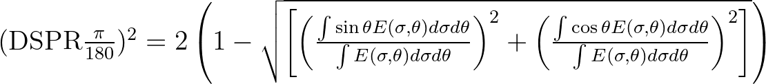
| DSPR | The one-sided directional width of the spectrum (directional spreading | |
| or directional standard deviation,in ), defined as |
||
 |
||
| and computed as conventionally for pitch-and-roll buoy data | ||
| (Kuik et al. (1988); this is the standard definition for WAVEC buoys | ||
| integrated over all frequencies): | ||
![$({\rm DSPR} \frac{\pi}{180})^2 = 2\left( 1 - \sqrt{\left[ \left( \frac{\int\sin...
...\sigma d\theta}{\int E(\sigma,\theta)d\sigma d\theta} \right)^2 \right]}\right)$](img175.png) |
||
| QP | The peakedness of the wave spectrum, defined as | |
 |
||
| This quantity represents the degree of randomness of the waves. | ||
A smaller value of 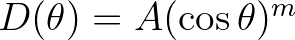 indicates a wider spectrum and thus indicates a wider spectrum and thus |
||
| increased the degree of randomness (e.g., shorter wave groups), | ||
| whereas a larger value indicates a narrower spectrum and a more | ||
| organised wave field (e.g., longer wave groups). | ||
| MS | As input to SWAN with the commands BOUNDPAR and BOUNDSPEC, | |
| the directional distribution | of incident wave energy is given by | |
 |
for all frequencies. The parameter  |
|
| is indicated as MS in SWAN and is not necessarily an integer number. | ||
| This number is related to the | one-sided directional spread of the waves | |
| (DSPR) as follows: |
| MS | DSPR (in ) |
|
| 1. | 37.5 | |
| 2. | 31.5 | |
| 3. | 27.6 | |
| 4. | 24.9 | |
| 5. | 22.9 | |
| 6. | 21.2 | |
| 7. | 19.9 | |
| 8. | 18.8 | |
| 9. | 17.9 | |
| 10. | 17.1 | |
| 15. | 14.2 | |
| 20. | 12.4 | |
| 30. | 10.2 | |
| 40. | 8.9 | |
| 50. | 8.0 | |
| 60. | 7.3 | |
| 70. | 6.8 | |
| 80. | 6.4 | |
| 90. | 6.0 | |
| 100. | 5.7 | |
| 200. | 4.0 | |
| 400. | 2.9 | |
| 800. | 2.0 |
| PROPAGAT | Energy propagation per unit time in  , ,  and and  space space |
|
(in W/ or /s, depending on the command SET). or /s, depending on the command SET). |
||
| GENERAT | Energy generation per unit time due to the wind input | |
| (in W/ or /s, depending on the command SET). |
||
| REDIST | Energy redistribution per unit time due to the sum of quadruplets | |
| and triads (in W/ or /s, depending on the command SET). |
||
| DISSIP | Energy dissipation per unit time due to the sum of bottom friction, | |
| whitecapping and depth-induced | surf breaking (in W/ or /s, |
|
| depending on the command SET). | ||
| RADSTR | Work done by the radiation stress per unit time, defined as | |
 |
||
| (in W/ or /s, depending on the command SET). |
||
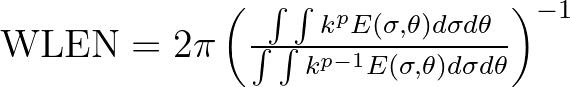
| WLEN | The mean wave length, defined as | |
 |
||
| As default, (see command QUANTITY). |
||
| STEEPNESS | Wave steepness computed as HSIG/WLEN. | |
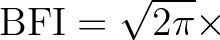
| BFI | The Benjamin-Feir index or the steepness-over-randomness ratio, | |
| defined as | ||
 STEEPNESS STEEPNESS  QP QP |
||
| This index can be used to quantify the probability of freak waves. | ||
| QB | Fraction of breakers in expression of Battjes and Janssen (1978). | |
| TRANSP | Energy transport with components
 and and |
|
 |
with  and and  the problem coordinate system, the problem coordinate system, |
|
| except in the case of output with BLOCK command in combination | ||
with command FRAME, where and relate to the  axis and axis and  axis axis |
||
| of the output frame. | ||
| VEL | Current velocity components in and direction of the problem |
|
| coordinate system, | except in the case of output with BLOCK command in | |
| combination with command FRAME, where and relate to the axis |
||
| and axis of the output frame. |
||
| WIND | Wind velocity components in and direction of the problem coordinate |
|
| sytem, except in the case of output with BLOCK command in | combination | |
| with command FRAME, where and relate to the axis and axis of |
||
| the output frame. | ||
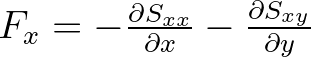
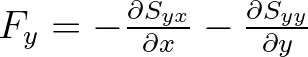
| FORCE | Wave-induced force per unit surface area (gradient of radiation stresses) | |
| with and the problem coordinate system, except in the case of output |
||
| with BLOCK command in | combination with command FRAME, | |
| where and relate to the axis and axis of the output frame. |
||
 |
||
 |
||
where  is the radiation stress tensor as given by is the radiation stress tensor as given by |
||
 |
||
 |
||
 |
||
and  is the group velocity over the phase velocity. is the group velocity over the phase velocity. |
||
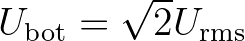
| UBOT | Root-mean-square value (in m/s) of the maxima of the orbital motion | |
near the bottom
 . . |
||
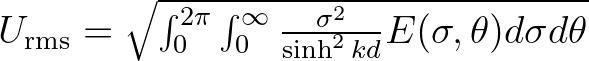
| URMS | Root-mean-square value (in m/s) of the orbital motion near the bottom. | |
 |
||
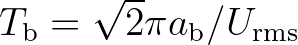
| TMBOT | Near bottom wave period (in s) defined as the ratio of the bottom excursion | |
amplitude to the root-mean-square velocity
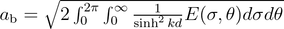 with with |
||
 |
||
| LEAK | Numerical loss of energy equal to
 across boundaries across boundaries  =[dir1] =[dir1] |
|
and  =[dir2] of a directional sector (see command CGRID). =[dir2] of a directional sector (see command CGRID). |
||
| TIME | Full date-time string. | |
| TSEC | Time in seconds with respect to a reference time (see command QUANTITY). | |
| SETUP | The elevation of mean water level (relative to still water level) induced by | |
| the gradient of the radiation stresses of the waves. | ||
| Cartesian convention | The direction is the angle between the vector and the positive axis, |
|
| measured counterclockwise. In other words: the direction where the | ||
| waves are going to or where the wind is blowing to. | ||
| Nautical convention | The direction of the vector from geographic North measured | |
| clockwise. In other words: the direction where the waves are coming | ||
| from or where the wind is blowing from. |
The SWAN team 2026-03-13