Next: Triads Up: Nonlinear wave-wave interactions () Previous: Nonlinear wave-wave interactions ()
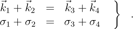
 is a coefficient with a default value of 0.25. To satisfy the resonance conditions for the first
quadruplet, the wave number vectors with frequency
is a coefficient with a default value of 0.25. To satisfy the resonance conditions for the first
quadruplet, the wave number vectors with frequency  and
and  lie at an angle of
 and
and
 to the angle of the wave number vectors with frequencies
  and
and  .
The second quadruplet is the mirror image of the first
quadruplet with relative angles of
.
The second quadruplet is the mirror image of the first
quadruplet with relative angles of
 and
and
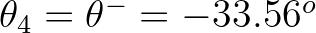 .
An example of this
wave number configuration is shown in Figure 2.2. See Van Vledder et al. (2000) for further
information about wave number configurations for arbitrary values of .
.
An example of this
wave number configuration is shown in Figure 2.2. See Van Vledder et al. (2000) for further
information about wave number configurations for arbitrary values of .
 |
 for the nonlinear transfer rate is given by
 refers to the first quadruplet and
 to the second quadruplet
(the expressions for
are identical to those for
for the mirror directions).
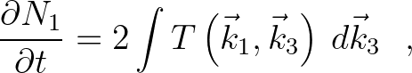
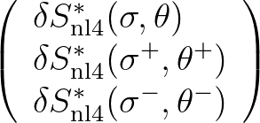
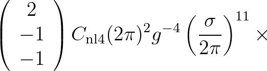
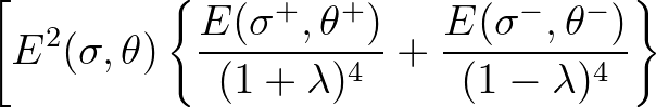
The DIA exchanges wave variance at all three wave number vectors involved in a quadruplet
wave number configuration. The rate of change of wave variance due to the quadruplet
interaction at the three frequency-direction bins can be written as
to the second quadruplet
(the expressions for
are identical to those for
for the mirror directions).
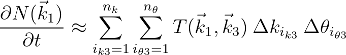
The DIA exchanges wave variance at all three wave number vectors involved in a quadruplet
wave number configuration. The rate of change of wave variance due to the quadruplet
interaction at the three frequency-direction bins can be written as
 by default.
Eq. (2.78) conserves wave variance, momentum and
action when the frequencies are geometrically distributed (as is the case in the SWAN
model). The wave variance density at the frequency-direction bins
by default.
Eq. (2.78) conserves wave variance, momentum and
action when the frequencies are geometrically distributed (as is the case in the SWAN
model). The wave variance density at the frequency-direction bins
 and
and
 is
obtained by bi-linear interpolation between the four surrounding frequency-direction bins.
Similarly, the rate of change of variance density is distributed between the four surrounding
bins using the same weights as used for the bi-linear interpolation.
is
obtained by bi-linear interpolation between the four surrounding frequency-direction bins.
Similarly, the rate of change of variance density is distributed between the four surrounding
bins using the same weights as used for the bi-linear interpolation.
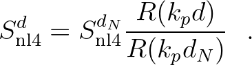
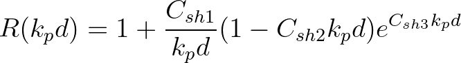
 is obtained by multiplying the deep water nonlinear transfer rate by a scaling factor
 :
:
 is given by
 is the peak wave number of the frequency spectrum. WAMDI (1988) proposes the
following values of the coefficients:
is the peak wave number of the frequency spectrum. WAMDI (1988) proposes the
following values of the coefficients:
 ,
,
 and
and
 .
In the shallow water limit, i.e.,
.
In the shallow water limit, i.e.,
 the nonlinear transfer rate tends to infinity. Therefore,
a lower limit of
the nonlinear transfer rate tends to infinity. Therefore,
a lower limit of  is applied, resulting in a maximum value
of
is applied, resulting in a maximum value
of  . To increase the model robustness in case of arbitrarily shaped spectra, the peak wave number
is replaced by
. To increase the model robustness in case of arbitrarily shaped spectra, the peak wave number
is replaced by
 (cf. Komen et al., 1994).
 at
wave number
at
wave number  due to all quadruplet interactions involving
is given by
due to all quadruplet interactions involving
is given by
 |
 |
 | ||
![$\displaystyle \hspace{7mm}\times \:\:\: \left[ {N_1 N_3 \left( {N_4 - N_2 } \ri...
...N_3 - N_1 } \right)} \right] \: d\vec{k}_2 \: d\vec{k}_3 \: d\vec{k}_4 \:\:\: ,$](img320.png) | (2.82) |
 is defined in terms of the wave number
vector
is defined in terms of the wave number
vector  ,
,
 . The term
  is a complicated coupling
coefficient for which an explicit expression has been given by Herterich and Hasselmann (1980).
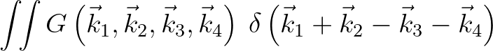
In the WRT method a number of transformations are
made to remove the delta functions. A key element in the WRT method
is to consider the integration space for each (
is a complicated coupling
coefficient for which an explicit expression has been given by Herterich and Hasselmann (1980).
In the WRT method a number of transformations are
made to remove the delta functions. A key element in the WRT method
is to consider the integration space for each (
 )
combination
)
combination
 (2.83)
 is given by
 (2.85)
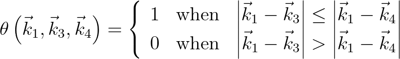
 determines a section of the integral which is
not defined due to the assumption that
is closer to
determines a section of the integral which is
not defined due to the assumption that
is closer to  than
than  . The crux of the Webb method
consists of using a local co-ordinate system along a so-named
locus, that is, the path in space that satisfies the resonance conditions for a given combination
of and . To that end the
. The crux of the Webb method
consists of using a local co-ordinate system along a so-named
locus, that is, the path in space that satisfies the resonance conditions for a given combination
of and . To that end the  co-ordinate system is
replaced by a
co-ordinate system is
replaced by a  co-ordinate system, where
  (
( ) is the tangential (normal) direction
along the locus. After some
transformations the transfer integral can then be written as a closed
line integral along the closed locus
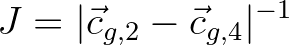
is the coupling coefficient and
) is the tangential (normal) direction
along the locus. After some
transformations the transfer integral can then be written as a closed
line integral along the closed locus
is the coupling coefficient and  is the Jacobian term of a function representing the resonance conditions.
The Jacobian term is a function of the group velocities of interacting wave
numbers
is the Jacobian term of a function representing the resonance conditions.
The Jacobian term is a function of the group velocities of interacting wave
numbers
 (2.87)
for all discrete combinations of and
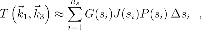
. The line integral (2.86) is solved by dividing the
locus in typically 40 pieces, such that its discretized version is
given by
(2.87)
for all discrete combinations of and
. The line integral (2.86) is solved by dividing the
locus in typically 40 pieces, such that its discretized version is
given by
 (2.88)
 is the product term for a given point on the locus,
 is the number of segments,
  is the discrete co-ordinate
along the locus, and
is the discrete co-ordinate
along the locus, and  is the stepsize. Finally, the rate
of change for a given wave number is given by
is the stepsize. Finally, the rate
of change for a given wave number is given by
 and
and  are the discrete number of wave numbers and
directions in the computational spectral grid, respectively. Note that although
the spectrum is defined in terms of the vector wave number , the
computational grid in a wave model is more conveniently defined in
terms of the absolute wave number and wave direction (
are the discrete number of wave numbers and
directions in the computational spectral grid, respectively. Note that although
the spectrum is defined in terms of the vector wave number , the
computational grid in a wave model is more conveniently defined in
terms of the absolute wave number and wave direction ( ) to
assure directional isotropy of the calculations. Taking all wave
numbers into account produces the complete source term due to
nonlinear quadruplet wave-wave interactions. Details of the
computation of a locus for a given combination of the wave numbers
and can be found in Van Vledder (2006).
) to
assure directional isotropy of the calculations. Taking all wave
numbers into account produces the complete source term due to
nonlinear quadruplet wave-wave interactions. Details of the
computation of a locus for a given combination of the wave numbers
and can be found in Van Vledder (2006).
 to
to  times more
computational effort than the DIA. Presently, these calculations can
therefore only be made for highly idealized test cases involving a
limited spatial grid.
times more
computational effort than the DIA. Presently, these calculations can
therefore only be made for highly idealized test cases involving a
limited spatial grid.
 grid which is based on the
 grid of SWAN.
In addition, the WRT routines inherit the power of the parametric
spectral tail as in the DIA. Choosing a higher resolution than the computational
grid of SWAN for computing the nonlinear interactions is possible in theory, but this
does not improve the results and is therefore not implemented.
grid of SWAN.
In addition, the WRT routines inherit the power of the parametric
spectral tail as in the DIA. Choosing a higher resolution than the computational
grid of SWAN for computing the nonlinear interactions is possible in theory, but this
does not improve the results and is therefore not implemented.
 . For
specific purposes other resolutions may be used, and some
testing with other resolutions may be needed.
. For
specific purposes other resolutions may be used, and some
testing with other resolutions may be needed.
 for which a valid BQF file has been generated.
In addition, the result is rescaled using the DIA scaling (2.80) according to
for which a valid BQF file has been generated.
In addition, the result is rescaled using the DIA scaling (2.80) according to
 (2.90)
The SWAN team 2026-03-13


![$\displaystyle \left. \left. -2\frac{E(\sigma,\theta) E(\sigma^+,\theta^+) E(\sigma^-,\theta^-)}{(1-\lambda^2)^4}
\right. \right]$](img300.png)


![$\displaystyle \left [ N_1 N_3 \left ( N_4 - N_2 \right ) + N_2 N_4 \left
(
N_3 - N_1 \right ) \right ] \: d\vec{k}_2 \: d\vec{k}_4 \:\:\: ,$](img330.png)
![$\displaystyle \left [ N_1 N_3 \left ( N_4 - N_2 \right ) + N_2 N_4 \left
(
N_3 - N_1 \right ) \right ] \: d s \:\:\: ,$](img337.png)