Next: Wave damping due to Up: Nonlinear wave-wave interactions () Previous: Quadruplets
This section outlines the computation of nonlinear interactions at shallow water by means of two methods.
The first method is based on a quadratic wave theory that express the nonlinear energy transfer using the
interaction coefficient. With this method, three different formulations will be discussed: the Full Triad
Interaction Model (FTIM), the Stochastic Parametric model based on Boussinesq equations (SPB) and the
Lumped Triad Approximation (LTA).
The second method is called the Discrete Collinear Triad Approximation (DCTA) method and heuristically
captures the  spectral tail at shallow water depths, while generating all transient sub and super harmonics.
Quadratic formulations
The starting point of the quadratic wave theory is to describe the free surface elevation of random spread but long-crested waves
propagating over a mildly sloping bed  using the following one-dimensional expression
(see, e.g. Freilich and Guza, 1984; Eldeberky, 1996; Herbers and Burton, 1997; Akrish et al, 2024)
using the following one-dimensional expression
(see, e.g. Freilich and Guza, 1984; Eldeberky, 1996; Herbers and Burton, 1997; Akrish et al, 2024)
![$\displaystyle \eta(x,t) = \sum_{p=-\infty}^{\infty} A_p(x)\,\exp{[{\rm i} (\omega_p t - \psi_p(x))]}
$](img356.png) (2.91)
(2.91)
 is the complex Fourier amplitude of the
  th harmonic,
  is the th
angular frequency and
is the th
angular frequency and  is the linear phase of th wave component with
 the wave number. The latter two numbers satisfy the linear dispersion relation:
 . Note that
 with
with  indicating the complex
conjugate and also
indicating the complex
conjugate and also
 and
and
 .
is a slow function of
.
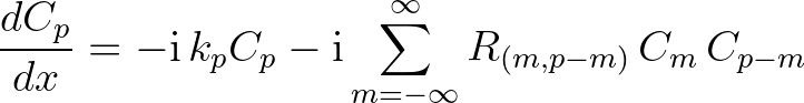
is a slow function of  due to shoaling and nonlinear interactions. Its evolution
equation is given by (Madsen and Sørensen, 1993; Eldeberky ,1996)
due to shoaling and nonlinear interactions. Its evolution
equation is given by (Madsen and Sørensen, 1993; Eldeberky ,1996)
![$\displaystyle \frac{dA_p}{dx} = -S_p A_p - {\rm i} \sum_{m=-\infty}^{\infty} R_{(m,p-m)}\,A_m\,A_{p-m}\,\exp{[-{\rm i}(\psi_m+\psi_{p-m}-\psi_p)]}
$](img368.png) (2.92)
(2.92)
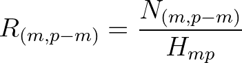
 the shoaling coefficient and
  the interaction coefficient. Note that
  is real and symmetric:
 with the subscripts
  and
and  denoting dummy indices.
Various expressions for the interaction coefficient will be discussed later.
The first and second term on the right hand side represent
linear shoaling and nonlinear triad interactions, respectively.
In the following we focus on the interaction term and therefore omit the shoaling part.
denoting dummy indices.
Various expressions for the interaction coefficient will be discussed later.
The first and second term on the right hand side represent
linear shoaling and nonlinear triad interactions, respectively.
In the following we focus on the interaction term and therefore omit the shoaling part.
![$\displaystyle C_p (x) = A_p (x) \exp{[-{\rm i}\,\psi_p(x)]}
$](img374.png) (2.93)
(2.93)
 from sum
interactions of two components
from sum
interactions of two components  and
and  and difference interactions between
  and , respectively, as follows
 (2.96)
 denotes the expected value. The third-order moment is known as the discrete bispectrum
(Hasselmann et al, 1963) and its definition is given by
denotes the expected value. The third-order moment is known as the discrete bispectrum
(Hasselmann et al, 1963) and its definition is given by
 (2.97)
 (2.98)
 to , as follows
 (2.100)
![\begin{eqnarray*}
\frac{dB_{m,p-m}}{dx} = &-& {\rm i}\,\Delta k\,B_{m,p-m} \non...
..._{(n,p-m-n)}\,T_{m,n,p-m-n} - R_{(n,m-n)}\,T_{n,m-n,p-m} \right]
\end{eqnarray*}](img386.png)
 is the wave number mismatch and
  is the fourth-order moment or the discrete trispectrum and is defined as
 (2.101)
 the Kronecker delta.
With respect to the cumulant term
the Kronecker delta.
With respect to the cumulant term  , the following two hypotheses are introduced: i) the quasi-Gaussian hypothesis (or the quasi-normal
closure) and the closure hypothesis of Holloway (1980).
, the following two hypotheses are introduced: i) the quasi-Gaussian hypothesis (or the quasi-normal
closure) and the closure hypothesis of Holloway (1980).
 .
With Eq. (2.102), the evolution equation of reduces to
.
With Eq. (2.102), the evolution equation of reduces to
![$\displaystyle \frac{dB_{m,p-m}}{dx} = -{\rm i}\,\Delta k\,B_{m,p-m} + 2\,{\rm i...
...p-m)}\,E_m\,E_{p-m} - R_{(p,-m)}\,E_m\,E_p - R_{(m-p,p)}\,E_{p-m}\,E_p \right]
$](img394.png) (2.103)
is proportional to , implying the following evolution equation for the bispectrum
(2.103)
is proportional to , implying the following evolution equation for the bispectrum
![\begin{eqnarray*}
\frac{dB_{m,p-m}}{dx} = &-& {\rm i}\,\Delta k\,B_{m,p-m}\nonu...
...{(m-p,p)}\,E_{p-m}\,E_p \right] \nonumber \\
&-& K\, B_{m,p-m}
\end{eqnarray*}](img395.png)
 an empirical parameter (unit: m
 ) which allows for relaxing the bispectrum towards a Gaussian state.
Note that this is rather a crude approximation since it does not account for the influence of the interaction coefficients.
) which allows for relaxing the bispectrum towards a Gaussian state.
Note that this is rather a crude approximation since it does not account for the influence of the interaction coefficients.
![$\displaystyle \frac{dB_{m,p-m}}{dx} = -{\rm i}\,\Psi\,B_{m,p-m} + 2\,{\rm i}
\...
...p-m)}\,E_m\,E_{p-m} - R_{(p,-m)}\,E_m\,E_p - R_{(m-p,p)}\,E_{p-m}\,E_p \right]
$](img398.png) (2.104)
(2.104)
![$\displaystyle B_{l,k} = \vert B_{l,k}\vert \, \exp{[-{\rm i} \beta_{l,k}]}
$](img402.png) (2.108)
(2.108)
 the bicoherence and
  the biphase.
Consequently, the evolution equation (2.99) for the discrete spectrum is rewritten as
the biphase.
Consequently, the evolution equation (2.99) for the discrete spectrum is rewritten as
 is a real number).
The above approach using the quasi-Gaussian hypothesis serves as the basis for modelling the spectral source term for triad interactions.
We come back to this point later. This also includes the parametrization of the biphase.
is a real number).
The above approach using the quasi-Gaussian hypothesis serves as the basis for modelling the spectral source term for triad interactions.
We come back to this point later. This also includes the parametrization of the biphase.
 the steady-state solution (2.107)
is a complex number and hence
the steady-state solution (2.107)
is a complex number and hence
![$\displaystyle {\rm Im}(B_{m,p-m}) = \frac{2K}{(\Delta k)^2+K^2}\,\left[ R_{(m,p-m)}\,E_m\,E_{p-m} - R_{(p,-m)}\,E_m\,E_p - R_{(m-p,p)}\,E_{p-m}\,E_p \right]
$](img409.png) (2.111)
(2.111)

 . To derive the spectral source
term for triads a relation between and the variance density spectrum
. To derive the spectral source
term for triads a relation between and the variance density spectrum  must be established. The single-sided variance density spectrum at frequency
  is given by
 (2.112)
 the th frequency step. Note that the frequency resolution may not be constant.
 consisting of quadratic products of variance density at different frequencies:
 (2.114)
 subharmonic transfers take place with a mismatch of 180
 in the biphase. This can be taken into account by just ignoring the absolute sign
of the
in the biphase. This can be taken into account by just ignoring the absolute sign
of the  function.
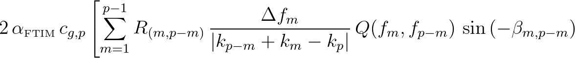
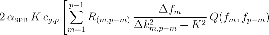
source term that conserves the energy flux
function.
source term that conserves the energy flux
 is obtained after multiplying the above result with a calibration factor
  and the
group velocity
and the
group velocity  , as follows
 will be
  .
.
 , etc. Again,
 .
.
 :
:
 (2.117)
 is the offshore peak wave number. However, Salmon (2016) argued the difficulty of defining in case of realistic applications
and suggested another expression that also prevents
is the offshore peak wave number. However, Salmon (2016) argued the difficulty of defining in case of realistic applications
and suggested another expression that also prevents  , namely,
 with
with  the local peak wave number. This is implemented in SWAN.
 .
.
 associated with each individual interaction is replaced by an effective interaction bandwidth
  .
is scaled with
.
is scaled with  and is scaled with . Hence, their ratio
 scales with
the phase speed
scales with
the phase speed  .
.
![$\displaystyle Q(f_m,f_{p-m}) = R_{(m,p-m)} \Bigl [E(f_m)\,E(f_{p-m}) - E(f_m)\,E(f_p) - E(f_{p-m})\,E(f_p)\Bigr ]
$](img445.png) (2.118)
(2.118)
![$\displaystyle Q(f_m,f_p) = R_{(m,p)} \Bigl [ E(f_m)\,E(f_p) - E(f_m)\,E(f_{p+m}) - E(f_p)\,E(f_{p+m}) \Bigr ]
$](img446.png) (2.119)
(2.119)
 (
( ) while replacing
  by the effective interaction bandwidth, as follows
 (2.120)
![$\displaystyle S^+_{\rm nl3} (f_p) = c_p \, R^2_{(p/2,p/2)} \, \max \Bigl [ \, 0,\,E^2(f_{p/2}) - 2\,E(f_{p/2})\,E(f_p) \, \Bigr ] \,\sin{(-\beta_{p/2,p/2})}
$](img451.png) (2.121)
due to self-self interaction at frequency .
(2.121)
due to self-self interaction at frequency .
 )
)
![$\displaystyle S^-_{\rm nl3} (f_p) = c_{2p} \, R^2_{(p,p)} \, \max \Bigl [ \, 0,\,E^2(f_p) - 2\,E(f_p)\,E(f_{2p}) \, \Bigr ] \,\sin{(-\beta_{p,p})}
$](img453.png) (2.122)
with itself leading to energy transfer to
(2.122)
with itself leading to energy transfer to  .
Note that
.
Note that
 which is the result of the first assumption. This further enhances the computational efficiency.
 is a tunable scaling factor that controls the strength of triad interactions.
 is computed only for frequencies
 with
with  the mean frequency (see Eq. 2.67).
A way to prevent this unwanted situation is to add another triad interaction, as outlined in the next section.
the mean frequency (see Eq. 2.67).
A way to prevent this unwanted situation is to add another triad interaction, as outlined in the next section.
 ,
,  and .
So, with
and .
So, with  and according to the first summation term of Eq. (2.115), the associated contribution of the sum interaction at reads
![$\displaystyle S^{++}_{\rm nl3} (f_p) = c_p \, R^2_{(2p/3,p/3)} \, \max \Bigl [ ...
...eft ( E(f_{p/3}) + E(f_{2p/3}) \right ) \, \Bigr ] \,\sin{(-\beta_{2p/3,p/3})}
$](img464.png) (2.124)
(2.124)
 and
and  to .
The contribution associated with the second term of Eq. (2.115) (difference interaction) is given by (
to .
The contribution associated with the second term of Eq. (2.115) (difference interaction) is given by ( )
)
![$\displaystyle S^{--}_{\rm nl3} (f_p) = c_{3p} \, R^2_{(2p,p)} \, \max \Bigl [ \...
...3p}) \, \left ( E(f_p) + E(f_{2p}) \right ) \, \Bigr ] \,\sin{(-\beta_{2p,p})}
$](img468.png) (2.125)
and
(2.125)
and  to
to  .
Again, notice that
.
Again, notice that
 .
.
 a calibration factor.
 where and are the dummy indices.
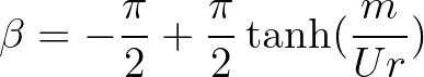
Instead of deriving an equation for the biphase (see, e.g. Reniers and Zijlema, 2022) a parametrization is proposed.
According to Eldeberky (1996), the biphase depends only on the spectral Ursell number, as follows
where and are the dummy indices.
Instead of deriving an equation for the biphase (see, e.g. Reniers and Zijlema, 2022) a parametrization is proposed.
According to Eldeberky (1996), the biphase depends only on the spectral Ursell number, as follows
 given by
a tunable coefficient. Note that there is no dependence on the wave frequencies, that is,
given by
a tunable coefficient. Note that there is no dependence on the wave frequencies, that is,
 for all and .
 based on a laboratory experiment.
However, our recent experience shows that this relatively low value triggers some instability that artificially amplifies higher
harmonics in the triad computation. Yet it will be less prone to error if the value of is increased.
As suggested by Doering and Bowen (1995), the optimal agreement of Eq. (2.127) with the data of some
field measurements is obtained with a value of
based on a laboratory experiment.
However, our recent experience shows that this relatively low value triggers some instability that artificially amplifies higher
harmonics in the triad computation. Yet it will be less prone to error if the value of is increased.
As suggested by Doering and Bowen (1995), the optimal agreement of Eq. (2.127) with the data of some
field measurements is obtained with a value of  , which also reflects a robust numerical performance.
 and
and  while the third component at is either a superharmonic or a subharmonic due to the (near) resonance condition.
The energy transfer is controlled by the interaction coefficient which is derived from a time-domain wave model.
Various formulations exist for the quadratic model and an overview is provided by Akrish et al (2024).
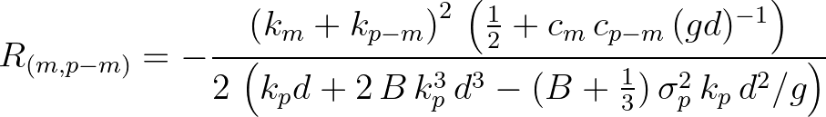
are implemented. In the earlier SWAN versions, the
interaction coefficient based on the Boussinesq-wave theory of Madsen and Sørensen (1993) was implemented for the purpose of the LTA
as proposed by Eldeberky (1996). The other three formulations are due to Freilich and Guza (1984), Bredmose et al (2005) and,
recently published in Akrish et al (2024), the QuadWave model. The four interaction coefficients are summarized below.
while the third component at is either a superharmonic or a subharmonic due to the (near) resonance condition.
The energy transfer is controlled by the interaction coefficient which is derived from a time-domain wave model.
Various formulations exist for the quadratic model and an overview is provided by Akrish et al (2024).
are implemented. In the earlier SWAN versions, the
interaction coefficient based on the Boussinesq-wave theory of Madsen and Sørensen (1993) was implemented for the purpose of the LTA
as proposed by Eldeberky (1996). The other three formulations are due to Freilich and Guza (1984), Bredmose et al (2005) and,
recently published in Akrish et al (2024), the QuadWave model. The four interaction coefficients are summarized below.
 (2.129)
 .
.
 (2.130)
 and
and  are the phase speed and the wave number, respectively, derived from the linear dispersion:
 .
Furthermore,
.
Furthermore,  .
.
 (2.131)
 (2.132)
 (2.133)
 and
and
 .
.
 (2.134)
 is the weight function defined as
![$\displaystyle W_{(m,p-m)} = \exp{\Biggl [-\left( \frac{\chi}{\alpha_3} \right)^{\alpha_2} \Biggr]}
$](img497.png) (2.135)
(2.135)
 (2.136)
 ,
,  and
and  are the optimization parameters.
This weight function optimizes the predictive accuracy associated with the nonlinear development of waves propagating through the coastal waters.
This is obtained in SWAN using the following values:
are the optimization parameters.
This weight function optimizes the predictive accuracy associated with the nonlinear development of waves propagating through the coastal waters.
This is obtained in SWAN using the following values:  ,
,
 and
and
 .
(Note that the original
.
(Note that the original  value of 1.4 yields too much energy in the high-frequency part of the spectrum.)
. The original expression for the Distributed Collinear Triad Approximation (DCTA) is given by
value of 1.4 yields too much energy in the high-frequency part of the spectrum.)
. The original expression for the Distributed Collinear Triad Approximation (DCTA) is given by
 (note that the frequencies match but the wave numbers not).
Here,
(note that the frequencies match but the wave numbers not).
Here,  is a calibration coefficient that controls the magnitude of triad interactions,
  is the parametrized biphase,
 with
with
 the mean frequency as given by Eq. (2.67),
  is a shape coefficient to force the high-frequency tail, and
 is a characteristic wave number of the triad.
Note that the factor
is a characteristic wave number of the triad.
Note that the factor
 in Eq. (2.137) accounts for the increasing resonance mismatch with increasing wave number (Booij et al., 2009).
 the transfer function of Sand (1982) and
 .
.
 .
.
The SWAN team 2026-03-13


![$\displaystyle B_{m,p-m} = \frac{2}{\Psi}\,\left[ R_{(m,p-m)}\,E_m\,E_{p-m} - R_{(p,-m)}\,E_m\,E_p - R_{(m-p,p)}\,E_{p-m}\,E_p \right]
$](img401.png)


![$\displaystyle \left. - 2\,\sum_{m=1}^{\infty} R_{(p+m,-m)} \, \frac{\Delta f_m}{\vert k_{p}+k_m-k_{p+m}\vert}\,
Q(f_m,f_p) \,\sin{(-\beta_{m,p})} \right]$](img427.png)
![$\displaystyle \left. - 2\,\sum_{m=1}^{\infty} R_{(p+m,-m)} \, \frac{\Delta f_m}{\Delta k^2_{m,p}+K^2}\,
Q(f_m,f_p) \right]$](img431.png)
![$\displaystyle S_{\rm nl3}(f_p) = \alpha_{\mbox{\tiny LTA}} \, c_{g,p} \left[ S^+_{\rm nl3} (f_p) - 2\, S^-_{\rm nl3} (f_p) \right]
$](img456.png)
![$\displaystyle S_{\rm nl3}(f_p) = \alpha_{\mbox{\tiny LTA+}} \, c_{g,p} \left[ S...
..._{\rm nl3} (f_p) + S^{++}_{\rm nl3} (f_p) - 2\, S^{--}_{\rm nl3} (f_p) \right]
$](img472.png)
![$\displaystyle S_{\rm nl3} (\sigma_1) = \lambda \, \frac{\sin(-\beta)\,\tilde{k}...
...,2}k_2^p\,N(\sigma_2) - \sigma_1\,c_{g,1}k_1^p\,N(\sigma_1) \Bigr] \,d\sigma_2
$](img506.png)
![$\displaystyle S_{\rm nl3} (\sigma_1) = \lambda \, c_{g,1}\frac{\sin(-\beta)\,\t...
...Bigl[ c_{g,2}k_2^p\,E(\sigma_2) - c_{g,1}k_1^p\,E(\sigma_1) \Bigr] \,d\sigma_2
$](img513.png)
![$\displaystyle \int_{0}^{2\pi} \int_{0}^{\infty} \biggl (\frac{\tanh\,\overline{...
..._2,\theta_2) - c_{g,1}k_1^p\,E(\sigma_1,\theta_1) \Bigr] \,d\sigma_2\,d\theta_2$](img515.png)