Next: Nonlinear wave-wave interactions () Up: Sources and sinks Previous: Input by wind ()
 )
)
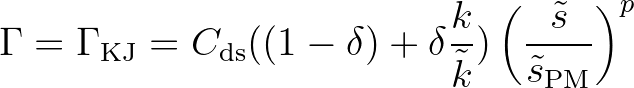
Whitecapping: Komen et al. (1984) formulation
The processes of whitecapping in the SWAN model is represented by the pulse-based model of
Hasselmann (1974). Reformulated in terms of wave number (rather than frequency) so as to be
applicable in finite water depth (cf. the WAMDI group, 1988), this expression is:
 and
and  denote the mean frequency and the mean wave number,
respectively, and the coefficient
denote the mean frequency and the mean wave number,
respectively, and the coefficient  depends on the overall wave steepness. This steepness dependent
coefficient, as given by the WAMDI group (1988), has been adapted by Günther et al. (1992) based on
Janssen (1991a) (see also (Janssen, 1991b)):
depends on the overall wave steepness. This steepness dependent
coefficient, as given by the WAMDI group (1988), has been adapted by Günther et al. (1992) based on
Janssen (1991a) (see also (Janssen, 1991b)):
 the expression of reduces to the expression as used by the WAMDI group (1988). The
coefficients
the expression of reduces to the expression as used by the WAMDI group (1988). The
coefficients  ,
,  and
and  are tunable coefficients,
  is the overall wave
steepness,
is the overall wave
steepness,
 is the value of for the Pierson-Moskowitz
spectrum (1964):
is the value of for the Pierson-Moskowitz
spectrum (1964):
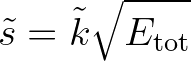
 . The overall wave steepness
is defined as
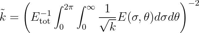
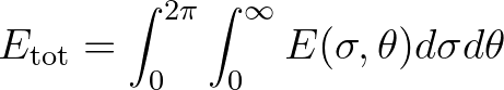
, the mean wave number and the total wave energy
. The overall wave steepness
is defined as
, the mean wave number and the total wave energy
 are defined as (cf. the WAMDI group, 1988):
and and exponent in this model have been obtained by
Komen et al. (1984) and Janssen (1992) by closing the energy balance of the waves in idealized wave growth conditions
(both for growing and fully developed wind seas) for deep water. This implies that coefficients in the steepness dependent
coefficient depend on the wind input formulation that is used. Since two different wind input formulations are
used in the SWAN model, two sets of coefficients are used. For the wind input of Komen et al. (1984; corresponding to WAM
Cycle 3; the WAMDI group, 1988):
are defined as (cf. the WAMDI group, 1988):
and and exponent in this model have been obtained by
Komen et al. (1984) and Janssen (1992) by closing the energy balance of the waves in idealized wave growth conditions
(both for growing and fully developed wind seas) for deep water. This implies that coefficients in the steepness dependent
coefficient depend on the wind input formulation that is used. Since two different wind input formulations are
used in the SWAN model, two sets of coefficients are used. For the wind input of Komen et al. (1984; corresponding to WAM
Cycle 3; the WAMDI group, 1988):
 , and
, and  . Janssen (1992) and also
Günther et al. (1992) obtained (assuming )
. Janssen (1992) and also
Günther et al. (1992) obtained (assuming )
 and
and  (as used in the WAM
Cycle 4; Komen et al., 1994).
from 0 to 1 leads to an improved prediction of the wave energy at lower frequencies.
Because of this, is set to 1 as default since version 40.91A.
However, it should be mentioned that adapting
without retuning
may lead to exceedence of the theoretical limits on wave height proposed by
Pierson and Moskowitz (1964).
(as used in the WAM
Cycle 4; Komen et al., 1994).
from 0 to 1 leads to an improved prediction of the wave energy at lower frequencies.
Because of this, is set to 1 as default since version 40.91A.
However, it should be mentioned that adapting
without retuning
may lead to exceedence of the theoretical limits on wave height proposed by
Pierson and Moskowitz (1964).
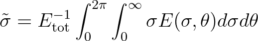
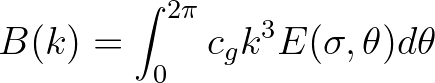
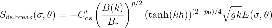
 is the azimuthal-integrated spectral saturation, which is positively correlated with
the probability of wave group-induced breaking. It is calculated from frequency space variables as follows
is the azimuthal-integrated spectral saturation, which is positively correlated with
the probability of wave group-induced breaking. It is calculated from frequency space variables as follows
 (2.51)
 is a threshold saturation level. The proportionality coefficient is set to
 . When
 , waves break and the exponent is set equal
to a calibration parameter
, waves break and the exponent is set equal
to a calibration parameter  . For
. For
 there is no breaking, but some residual dissipation proved
necessary. This is obtained by setting
there is no breaking, but some residual dissipation proved
necessary. This is obtained by setting  . A smooth transition between these two situations is achieved by
(Alves and Banner, 2003)
is simply set to (see below).
. A smooth transition between these two situations is achieved by
(Alves and Banner, 2003)
is simply set to (see below).
 is the contribution by breaking waves (2.50), and
 dissipation
by means other than breaking (e.g. turbulence). The changeover between the two modes is made with a smooth transition
function
dissipation
by means other than breaking (e.g. turbulence). The changeover between the two modes is made with a smooth transition
function  similar to (2.52):
, to provide general
background dissipation of non-breaking waves. For this component, the parameter settings of Komen et al. (1984)
are applied.
similar to (2.52):
, to provide general
background dissipation of non-breaking waves. For this component, the parameter settings of Komen et al. (1984)
are applied.
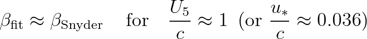
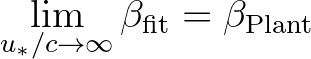
 say, the wind-induced growth rate of waves depends quadratically on
 (e.g. Plant 1982), whereas for weaker forcing,
  say, the growth rate depends linearly on
(Snyder et al., 1981). Yan (1987) proposes an analytical fit through these two ranges of the form:
say, the growth rate depends linearly on
(Snyder et al., 1981). Yan (1987) proposes an analytical fit through these two ranges of the form:
 ,
, ,
, and
and  are coefficients of the fit. Yan imposed two constraints:
 and
and
 are the growth rates proposed by Snyder et al. (1981) and Plant (1982), respectively.
Application of Eqs. (2.56) and (2.57) led us to parameter values of
are the growth rates proposed by Snyder et al. (1981) and Plant (1982), respectively.
Application of Eqs. (2.56) and (2.57) led us to parameter values of
 ,
,
 ,
,
 and
and
 , which are somewhat different from those proposed by Yan (1987). We found that our parameter values produce better
fetch-limited simulation results in the Pierson and Moskowitz (1964) fetch range thant the original values of Yan (1987).
in Eqs. (2.50) and (2.52) is made by requiring that the source terms of whitecapping
(Eq. 2.50) and wind input (Eq. 2.55) have equal scaling in frequency, after Resio et al. (2004). This leads to a value of
, which are somewhat different from those proposed by Yan (1987). We found that our parameter values produce better
fetch-limited simulation results in the Pierson and Moskowitz (1964) fetch range thant the original values of Yan (1987).
in Eqs. (2.50) and (2.52) is made by requiring that the source terms of whitecapping
(Eq. 2.50) and wind input (Eq. 2.55) have equal scaling in frequency, after Resio et al. (2004). This leads to a value of
 for strong wind forcing () and
  for weaker forcing (). A smooth transition between these two limits,
centred around
for weaker forcing (). A smooth transition between these two limits,
centred around  , is achieved by the expression
 is a scaling parameter for which a value of
  is used in SWAN. In shallow water, under strong wind forcing (), this
scaling condition requires the additional dimensionless factor
is used in SWAN. In shallow water, under strong wind forcing (), this
scaling condition requires the additional dimensionless factor
 in Eq. (2.50), where
  is the water depth.
 (2.13):
![$\displaystyle S_{\rm wc,curr} (\sigma,\theta) = -C''_{\rm ds} \max \left [ \fra...
...ma}, 0 \right ] \,\left( \frac{B(k)}{B_{\rm r}} \right)^{p/2} E(\sigma,\theta)
$](img227.png) (2.59)
(2.59)
 = 0.8. The remaining parameters are given by
Van der Westhuysen (2007), namely
and
= 0.8. The remaining parameters are given by
Van der Westhuysen (2007), namely
and  according to (2.58).
 (WW3) starting in 2010, and this
implementation was documented in Zieger et al. (2015). Since 2010, developments in the two models have largely
paralleled each other, insofar as most notable improvements are implemented in both models. As such, the documentation for WW3
(public release versions 4 or 5) is largely adequate documentation of significant changes to the source terms in SWAN since
the publication of Rogers et al. (2012), and do not need to be repeated here. We point out three notable exceptions to
this.
(WW3) starting in 2010, and this
implementation was documented in Zieger et al. (2015). Since 2010, developments in the two models have largely
paralleled each other, insofar as most notable improvements are implemented in both models. As such, the documentation for WW3
(public release versions 4 or 5) is largely adequate documentation of significant changes to the source terms in SWAN since
the publication of Rogers et al. (2012), and do not need to be repeated here. We point out three notable exceptions to
this.
 , following Komen et al. (1984), has been replaced with
 , where
  is a free parameter. Use of
  (we use
  )
yields significant improvements to the tail level, correcting overprediction mean square slope. This necessitates
tuning of the
)
yields significant improvements to the tail level, correcting overprediction mean square slope. This necessitates
tuning of the  and
and  coefficients. Settings are suggested in the SWAN User Manual. At time of writing, this
feature has not yet been ported to WW3.
coefficients. Settings are suggested in the SWAN User Manual. At time of writing, this
feature has not yet been ported to WW3.
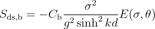
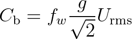
 is a bottom friction coefficient that generally depends on the bottom orbital motion
represented by
is a bottom friction coefficient that generally depends on the bottom orbital motion
represented by  :
:
 m
m s
s which is in
agreement with the JONSWAP result for swell dissipation. However, Bouws and Komen (1983) suggest a
value of
which is in
agreement with the JONSWAP result for swell dissipation. However, Bouws and Komen (1983) suggest a
value of
 ms for depth-limited wind-sea conditions in the North Sea. This value is derived
from revisiting the energy balance equation employing an alternative deep water dissipation.
Recently, in Zijlema et al. (2012) it was found that a unified value of
ms for depth-limited wind-sea conditions in the North Sea. This value is derived
from revisiting the energy balance equation employing an alternative deep water dissipation.
Recently, in Zijlema et al. (2012) it was found that a unified value of  ms can be used if the
second order polyomial fit for wind drag of Eq. (2.36) is employed.
So, in SWAN 41.01 this is default irrespective of swell and wind-sea conditions.
ms can be used if the
second order polyomial fit for wind drag of Eq. (2.36) is employed.
So, in SWAN 41.01 this is default irrespective of swell and wind-sea conditions.
 with
with  (Collins, 1972)2.2.
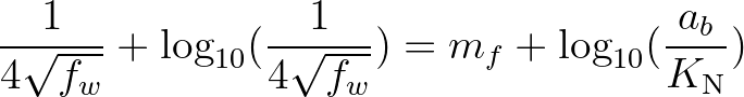
 is a non-dimensional friction factor estimated by using the formulation of Jonsson (1966) cf.
Madsen et al. (1988):
is a non-dimensional friction factor estimated by using the formulation of Jonsson (1966) cf.
Madsen et al. (1988):
 (Jonsson and Carlsen, 1976) and
  is a representative near-bottom excursion
amplitude:
is a representative near-bottom excursion
amplitude:
 is the bottom roughness length scale. For values of
  smaller than 1.57 the
friction factor is 0.30 (Jonsson, 1980).
smaller than 1.57 the
friction factor is 0.30 (Jonsson, 1980).
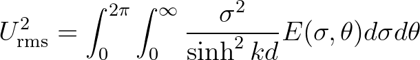
 is expressed as
 in SWAN,
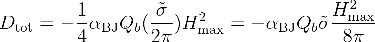
  is the fraction of breaking waves determined by
 is the maximum wave height that can exist at the given depth and
is a mean frequency defined as
) is determined in SWAN with
is the maximum wave height that can exist at the given depth and
is a mean frequency defined as
) is determined in SWAN with
 . Furthermore, for
 ,
,  and for
 ,
,
 .
is determined in SWAN with
.
is determined in SWAN with
 , in which
  is the breaker parameter
and
is the breaker parameter
and  is the total water depth (including the wave-induced set-up if computed by SWAN). In the literature,
this breaker parameter is often a constant or it is expressed as a function of bottom slope or incident
wave steepness (see e.g., Galvin, 1972; Battjes and Janssen, 1978; Battjes and Stive, 1985; Arcilla and
Lemos, 1990; Kaminsky and Kraus, 1993; Nelson, 1987, 1994).
In the publication of Battjes and Janssen (1978) in which the dissipation model is described, a constant
breaker parameter, based on Miche's criterion, of
is the total water depth (including the wave-induced set-up if computed by SWAN). In the literature,
this breaker parameter is often a constant or it is expressed as a function of bottom slope or incident
wave steepness (see e.g., Galvin, 1972; Battjes and Janssen, 1978; Battjes and Stive, 1985; Arcilla and
Lemos, 1990; Kaminsky and Kraus, 1993; Nelson, 1987, 1994).
In the publication of Battjes and Janssen (1978) in which the dissipation model is described, a constant
breaker parameter, based on Miche's criterion, of  was used. Battjes and Stive (1985) re-analyzed
wave data of a number of laboratory and field experiments and found values for the breaker parameter
varying between 0.6 and 0.83 for different types of bathymetry (plane, bar-trough and bar) with an average
of 0.73. From a compilation of a large number of experiments Kaminsky and Kraus (1993) have found
breaker parameters in the range of 0.6 to 1.59 with an average of 0.79.
was used. Battjes and Stive (1985) re-analyzed
wave data of a number of laboratory and field experiments and found values for the breaker parameter
varying between 0.6 and 0.83 for different types of bathymetry (plane, bar-trough and bar) with an average
of 0.73. From a compilation of a large number of experiments Kaminsky and Kraus (1993) have found
breaker parameters in the range of 0.6 to 1.59 with an average of 0.79.
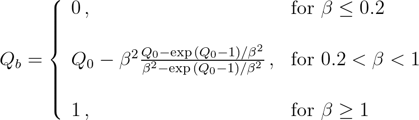
 is a proportionality coefficient and
  is the probability density function of breaking
waves times the fraction of breakers, . Based on field observations, the wave heights in the surf zone
are assumed to remain Rayleigh distributed, even after breaking. This implies that all waves will break, not
only the highest as assumed by Battjes and Janssen (1978). The function is obtained by multiplying
the Rayleigh wave height probability density function
is the probability density function of breaking
waves times the fraction of breakers, . Based on field observations, the wave heights in the surf zone
are assumed to remain Rayleigh distributed, even after breaking. This implies that all waves will break, not
only the highest as assumed by Battjes and Janssen (1978). The function is obtained by multiplying
the Rayleigh wave height probability density function  , given by
 (2.71)
 defined so that
 , to yield
 (2.72)
 (2.73)
 (=4) and a breaker index (not to be confused with the Battjes and Janssen breaker index!).
The integral in expression (2.70) can then be simplified, as follows
(=4) and a breaker index (not to be confused with the Battjes and Janssen breaker index!).
The integral in expression (2.70) can then be simplified, as follows
 (2.74)
The SWAN team 2026-03-13

![$\displaystyle p = \frac{p_0}{2} + \frac{p_0}{2} \tanh \left[ 10 \left( \sqrt{\frac{B(k)}{B_{\rm r}}} - 1 \right) \right]
$](img198.png)
![$\displaystyle S_{\rm ds,w}(\sigma,\theta) = f_{\rm br}(\sigma)S_{\rm ds,break} + \left[ 1 - f_{\rm br}(\sigma) \right]
S_{\rm ds,non-break} \ ,
$](img199.png)
![$\displaystyle f_{\rm br}(\sigma) = \frac{1}{2} + \frac{1}{2} \tanh \left[ 10 \left( \sqrt{\frac{B(k)}{B_{\rm r}}} - 1 \right) \right]
$](img203.png)

![$\displaystyle p_0(\sigma) = 3 + \tanh \left[ w \left( \frac{u_*}{c} - 0.1 \right) \right]
$](img221.png)