Next: Dissipation of wave energy Up: Sources and sinks Previous: General concepts
 )
)
Wave growth by wind is described by
 describes linear growth and
  exponential growth. It should be noted that the SWAN model
is driven by the wind speed at 10m elevation
exponential growth. It should be noted that the SWAN model
is driven by the wind speed at 10m elevation  whereas it uses the friction velocity
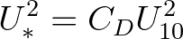
 . For the WAM Cycle 3 formulation the transformation from to is obtained with
 is the drag coefficient from Wu (1982):
 20 m/s, say).
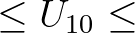
Based on many authoritative studies it appears that the drag coefficient increases almost linearly with wind speed up to approximately
20 m/s, then levels off and decreases again at about 35 m/s to rather low values at 60 m/s wind speed.
We fitted a 2nd order polynomial to the data obtained from these studies, and this fit is given by
20 m/s, say).
Based on many authoritative studies it appears that the drag coefficient increases almost linearly with wind speed up to approximately
20 m/s, then levels off and decreases again at about 35 m/s to rather low values at 60 m/s wind speed.
We fitted a 2nd order polynomial to the data obtained from these studies, and this fit is given by
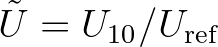 , and the reference wind speed
  = 31.5 m/s is the speed at which the drag attains its maximum value
in this expression. These drag values are lower than in the expression of Wu (1982) by 10%
= 31.5 m/s is the speed at which the drag attains its maximum value
in this expression. These drag values are lower than in the expression of Wu (1982) by 10%  30% for high wind speeds
(15
30% for high wind speeds
(15
 30 m/s) and over 30% for hurricane wind speeds ( 30 m/s). More details can be found in Zijlema et al. (2012).
Since version 41.01, the SWAN model employs the drag formulation as given by Eq. (2.36).
is an integral part of the source term.
, the expression due to Cavaleri and Malanotte-Rizzoli (1981) is used with a
filter to eliminate wave growth at frequencies lower than the Pierson-Moskowitz frequency (Tolman,
1992a)2.1:
30 m/s) and over 30% for hurricane wind speeds ( 30 m/s). More details can be found in Zijlema et al. (2012).
Since version 41.01, the SWAN model employs the drag formulation as given by Eq. (2.36).
is an integral part of the source term.
, the expression due to Cavaleri and Malanotte-Rizzoli (1981) is used with a
filter to eliminate wave growth at frequencies lower than the Pierson-Moskowitz frequency (Tolman,
1992a)2.1:
 is the wind direction,
  is the filter and
 is the peak frequency of the
fully developed sea state according to Pierson and Moskowitz (1964) as reformulated in terms of friction velocity.
is the peak frequency of the
fully developed sea state according to Pierson and Moskowitz (1964) as reformulated in terms of friction velocity.
 :
:
 is the phase speed and
  and
and  are the density of air and water, respectively. This
expression is also used in WAM Cycle 3 (the WAMDI group, 1988). The second expression is due to Janssen (1989,1991a).
It is based on a quasi-linear wind-wave theory and is given by
are the density of air and water, respectively. This
expression is also used in WAM Cycle 3 (the WAMDI group, 1988). The second expression is due to Janssen (1989,1991a).
It is based on a quasi-linear wind-wave theory and is given by
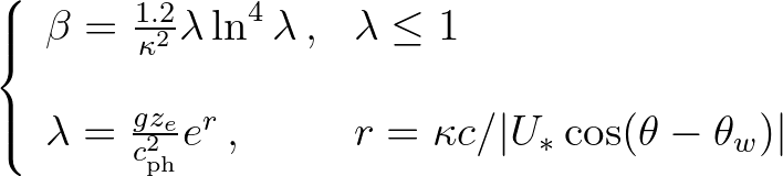
 is the Miles constant. In the theory of Janssen (1991a), this constant is estimated from
the non-dimensional critical height
is the Miles constant. In the theory of Janssen (1991a), this constant is estimated from
the non-dimensional critical height  :
:
 is the Von Karman constant and
  is the effective surface roughness.
If the non-dimensional critical height
is the effective surface roughness.
If the non-dimensional critical height  , the Miles constant is set equal 0.
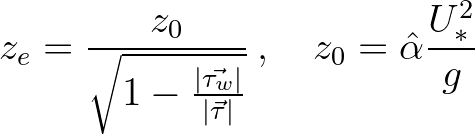
Janssen (1991a) assumes that the wind profile is given by
, the Miles constant is set equal 0.
Janssen (1991a) assumes that the wind profile is given by
 is the wind speed at height
  (10m in the SWAN model) above the mean water level,
  is
the roughness length. The effective roughness length depends on the roughness length and the sea
state through the wave-induced stress
is
the roughness length. The effective roughness length depends on the roughness length and the sea
state through the wave-induced stress  and the total surface stress
 :
:
 is a constant equal to 0.01. The
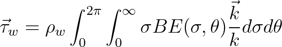
wave stress
is a constant equal to 0.01. The
wave stress  is given by
 can be determined for a given wind speed and a given wave spectrum
 from the
above set of equations. In the SWAN model, the iterative procedure of Mastenbroek et al. (1993) is used.
This set of expressions (2.39) through (2.43) is also used in WAM Cycle 4 (Komen et al., 1994).
from the
above set of equations. In the SWAN model, the iterative procedure of Mastenbroek et al. (1993) is used.
This set of expressions (2.39) through (2.43) is also used in WAM Cycle 4 (Komen et al., 1994).
The SWAN team 2026-03-13


![$\displaystyle B = \max [0, 0.25 \frac{\rho_a}{\rho_w} (28 \frac{U_*}{c_{\rm ph}}\cos(\theta-\theta_w) -1)]\sigma
$](img153.png)
![$\displaystyle B = \beta \frac{\rho_a}{\rho_w} \left(\frac{U_*}{c_{\rm ph}} \right)^2 \max[0,\cos(\theta-\theta_w)]^2\sigma
$](img156.png)
![$\displaystyle U(z) = \frac{U_*}{\kappa} \ln [ \frac{z+z_e-z_0}{z_e} ]
$](img162.png)