Next: Wave damping due to Up: Sources and sinks Previous: Triads
SWAN has an option to include
wave damping over a vegetation field (mangroves, salt marshes, etc.) at variable depths.
A popular method of expressing the wave dissipation due to vegetation is the cylinder approach
as suggested by Dalrymple et al. (1984). Here,
energy losses are calculated as actual work carried out by the vegetation due to plant
induced forces acting on the fluid, expressed in terms of a Morison type equation.
In this method, vegetation motion such as vibration due to vortices and swaying is
neglected. For relatively stiff plants the drag force is considered dominant and inertial
forces are neglected. Moreover, since the drag due to friction is much smaller than the
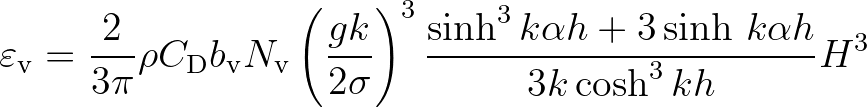
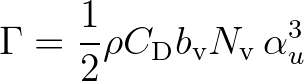
drag due to pressure differences, only the latter is considered. Based on
this approach, the time-averaged rate of energy dissipation per unit
area over the entire height of the vegetation is given by
 (2.139)
 is the water density,
  is the drag coefficient,
  is the
stem diameter of cylinder (plant),
is the
stem diameter of cylinder (plant),  is the number of plants per square meter,
 is the vegetation height,
  is the water depth and
  is the wave height.
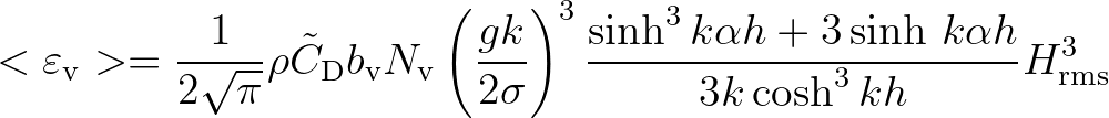
This formula was modified by Mendez and Losada (2004) for irregular waves.
The mean rate of energy dissipation per unit horizontal
area due to wave damping by vegetation is given by
is the wave height.
This formula was modified by Mendez and Losada (2004) for irregular waves.
The mean rate of energy dissipation per unit horizontal
area due to wave damping by vegetation is given by
 is the bulk drag coefficient that may depend on the wave height. This is the only
calibration parameter required for a given plant type.
is the bulk drag coefficient that may depend on the wave height. This is the only
calibration parameter required for a given plant type.
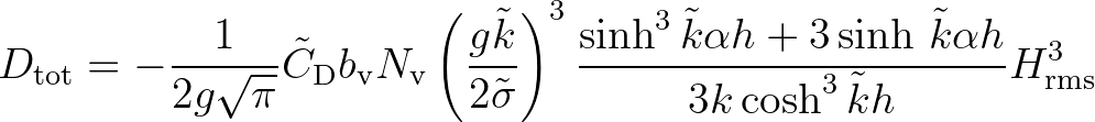
 based
on Eq. (2.141). A spectral version of the vegetation dissipation model of Mendez and
Losada can be obtained by expanding Eq. (2.141) to include frequencies and directions as
follows
based
on Eq. (2.141). A spectral version of the vegetation dissipation model of Mendez and
Losada can be obtained by expanding Eq. (2.141) to include frequencies and directions as
follows
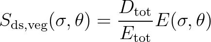 (2.141)
 , the mean wave number
  are given by Eqs. (2.47) and (2.48), respectively.
With
are given by Eqs. (2.47) and (2.48), respectively.
With
 , the final expression reads
 (2.143)
 (2.144)
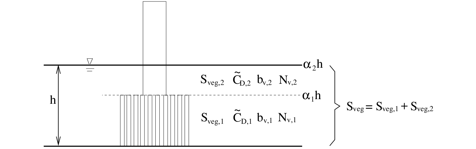
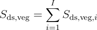
 the number of vegetation
layers and
the number of vegetation
layers and  the layer under consideration with the energy dissipation for layer .
First, a check is performed to establish whether the vegetation is emergent or submergent
relative to the water depth. In case of submergent vegetation the energy contributions of
each layer are added up for the entire vegetation height. In case of emergent vegetation
only the contributions of the layers below the still water level are taken into account.
The implementation of vertical variation is illustrated in Figure 2.3.
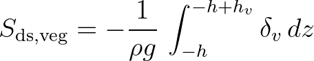
The energy dissipation term for a given layer therefore becomes
the layer under consideration with the energy dissipation for layer .
First, a check is performed to establish whether the vegetation is emergent or submergent
relative to the water depth. In case of submergent vegetation the energy contributions of
each layer are added up for the entire vegetation height. In case of emergent vegetation
only the contributions of the layers below the still water level are taken into account.
The implementation of vertical variation is illustrated in Figure 2.3.
The energy dissipation term for a given layer therefore becomes
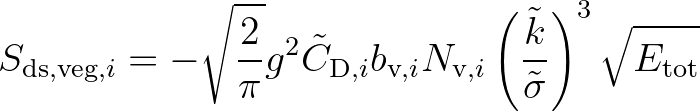 | ||||
 | (2.145) |
is the total water depth and  the ratio of the depth of the layer under
consideration to the total water depth up to the still water level, such that
the ratio of the depth of the layer under
consideration to the total water depth up to the still water level, such that
 (2.146)
, and are used in a linear way,
we can use as a control parameter to vary the vegetation factor
(2.146)
, and are used in a linear way,
we can use as a control parameter to vary the vegetation factor
 spatially, by setting
 and
and
 , so that
 .
.
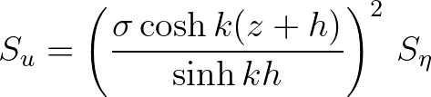
 (2.147)
 is the velocity spectrum
 (2.148)
 the energy density spectrum, i.e.
  .
The zeroth moment of the velocity spectrum is computed as
.
The zeroth moment of the velocity spectrum is computed as
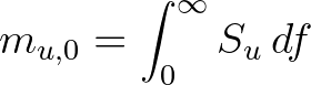 (2.149)
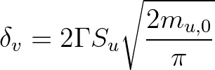
 (2.150)
 a velocity reduction factor.
 (2.151)
 the canopy height. The vertical integration is approximated using the Simpson's rule.
The SWAN team 2026-03-13