Next: Propagation of wave energy Up: Governing equations Previous: Governing equations
Wind generated waves have irregular wave heights and periods, caused by the irregular
nature of wind. Due to this irregular nature, the sea surface is continually varying,
which means that a deterministic approach to describe the sea surface is not feasible.
On the other hand, statistical properties of the surface, like average wave
height, wave periods and directions, appear to vary slowly in time and space, compared
to typical wave periods and wave lengths.
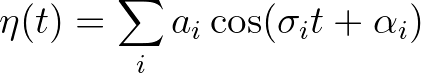
The surface elevation of waves in the ocean, at any location and any time,
can be seen as the sum of a large number of harmonic waves, each of which has been
generated by turbulent wind in different places and times. They are therefore
statistically independent in their origin. According to linear wave theory, they remain
independent during their journey across the ocean. Under these conditions, the sea
surface elevation on a time scale of hundreds of characterstic wave periods is sufficiently
well described as a stationary, Gaussian process. The sea surface elevation in one point as
a function of time can be described as
 the sea surface elevation,
  the random amplitude of the
  wave component,
 the relative radian or circular frequency of the wave component in the
presence of the ambient current (equals the absolute radian frequency
the relative radian or circular frequency of the wave component in the
presence of the ambient current (equals the absolute radian frequency  when no ambient
current is present) and
when no ambient
current is present) and  the random phase of the wave component.
This is called the random-phase model (Holthuijsen, 2007). Note that the random variables and
are characterized by their probability density functions; the amplitude of each wave component is Rayleigh
distributed and the phase of each component is uniformly distributed between 0 and 2
the random phase of the wave component.
This is called the random-phase model (Holthuijsen, 2007). Note that the random variables and
are characterized by their probability density functions; the amplitude of each wave component is Rayleigh
distributed and the phase of each component is uniformly distributed between 0 and 2 .
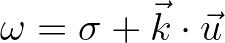
then equals the sum of
the relative radian frequency
.
then equals the sum of
the relative radian frequency  and the inner product of the wave number and ambient current
velocity vectors, as follows
and the inner product of the wave number and ambient current
velocity vectors, as follows
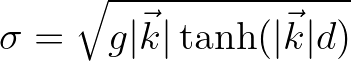
 and for linear waves the relative
frequency is given by
and for linear waves the relative
frequency is given by
 is the acceleration of gravity and
  is the water depth.
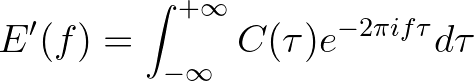
 the frequency (in Hz) and
 is the auto-covariance function,
  represents ensemble average of a random
variable,
represents ensemble average of a random
variable,  is the time lag and
  ,
,  describe two random processes of sea
surface elevation.
describe two random processes of sea
surface elevation.
 different
from the above one, as follows
different
from the above one, as follows
 (2.6)
is called spectral
description of water waves. This description is complete in a statistical sense under the assumption that
the sea surface is considered as a stationary, Gaussian random process.
should therefore
be interpreted as a variance density. The dimension of is m
(2.6)
is called spectral
description of water waves. This description is complete in a statistical sense under the assumption that
the sea surface is considered as a stationary, Gaussian random process.
should therefore
be interpreted as a variance density. The dimension of is m /Hz if the surface elevation is given
in meters and the frequency in Hz.
/Hz if the surface elevation is given
in meters and the frequency in Hz.
 is closely linked to the total energy
  of the waves per unit surface area,
as follows
of the waves per unit surface area,
as follows
 the water density.
The terms variance and energy density spectrum will therefore be
used indiscriminately in this document (however, see Zijlema, 2021).
the water density.
The terms variance and energy density spectrum will therefore be
used indiscriminately in this document (however, see Zijlema, 2021).
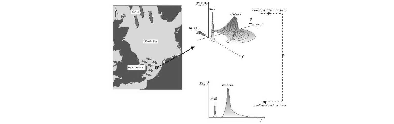
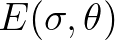
 and directions
  , is denoted by
  . Again, this
spectrum is assumed to provide a complete spectral description of the wave field if this field is
statistically quasi-homogeneous (and stationary Gaussian), which especially holds for broad-banded directional
waves (i.e. wind sea).
Section 2.7 discusses the extension of this description to include the statistical inhomogeneity
of the wave field (e.g. due to wave interference patterns).
is distributed over the directions in , it follows that
and are depicted in Figure 2.1.
. Again, this
spectrum is assumed to provide a complete spectral description of the wave field if this field is
statistically quasi-homogeneous (and stationary Gaussian), which especially holds for broad-banded directional
waves (i.e. wind sea).
Section 2.7 discusses the extension of this description to include the statistical inhomogeneity
of the wave field (e.g. due to wave interference patterns).
is distributed over the directions in , it follows that
and are depicted in Figure 2.1.
 |
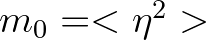
Based on the energy density spectrum, the integral wave parameters can be obtained. These parameters can be expressed in terms of the so-called
 th moment of the energy density spectrum
 . Well-known parameters are the significant
wave height
. Well-known parameters are the significant
wave height
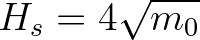 (2.11)
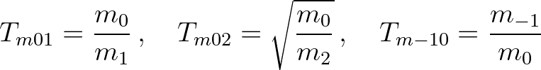 (2.12)
 is generally used. On a larger scale the spectral energy density
function
becomes a function of space and time, that is,
is generally used. On a larger scale the spectral energy density
function
becomes a function of space and time, that is,
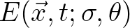 and wave dynamics should be considered to determine
the evolution of the spectrum in space and time.
and wave dynamics should be considered to determine
the evolution of the spectrum in space and time.
The SWAN team 2026-03-13