Computational grid

       | -> REGular [xpc] [ypc] [alpc] [xlenc] [ylenc] [mxc] [myc] |
       |                                                           |
CGRID <     CURVilinear [mxc] [myc]  (EXCeption  [xexc]  [yexc])    >  &
       |                                                           |
       |    UNSTRUCtured                                           |

          | -> CIRcle               |
         <                           > [mdc] [flow] [fhigh] [msc]
          |    SECtor [dir1] [dir2] |

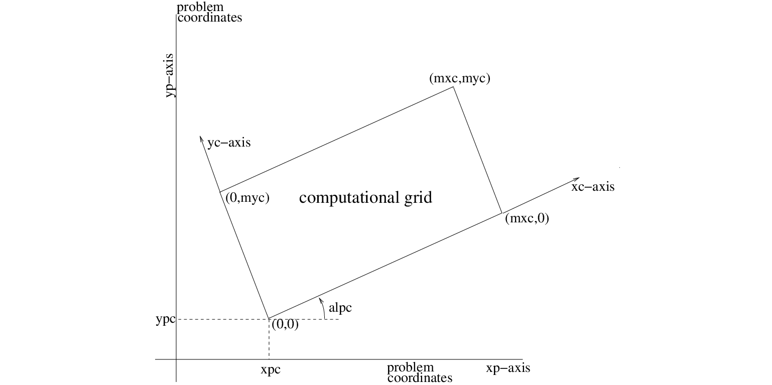
With this required command the user defines the geographic location, size, resolution and orientation of the computational grid in the problem coordinate system (see Section 2.6.3) in case of a uniform, rectilinear computational grid, a curvilinear grid or unstructured mesh. The origin of the regular grid and the direction of the positive $x-$axis of this grid can be chosen arbitrary by the user. Must be used for nested runs. Note that in a nested case, the geographic and spectral range (directional sector inclusive) and resolution may differ from the previous run (outside these ranges zero's are used).

REGULAR	this option indicates that the computational grid is to be taken as uniform and
	rectangular.
CURVILINEAR	this option indicates that the computational grid is to be taken as curvilinear.
	The user must provide the coordinates of the grid points with command
	READGRID COOR.
UNSTRUCTURE	this option indicates that the computational grid is to be taken as unstructured.
	The user must provide the coordinates of the vertices and the numbering of
	triangles with the associated connectivity table with vertices with command
	READGRID UNSTRUC.
[xpc]	geographic location of the origin of the computational grid in the problem
	coordinate system ($x-$coordinate, in m). See command COORD.
	Default: [xpc] = 0.0 (Cartesian coordinates).
	In case of spherical coordinates there is no default, the user must give a value.
[ypc]	geographic location of the origin of the computational grid in the problem
	coordinate system ($y-$coordinate, in m). See command COORD.
	Default: [ypc] = 0.0 (Cartesian coordinates).
	In case of spherical coordinates there is no default, the user must give a value.
[alpc]	direction of the positive $x-$axis of the computational grid (in degrees, Cartesian
	convention). In 1D-mode, [alpc] should be equal to the direction [alpinp]
	(see command INPGRID).
	Default: [alpc] = 0.0.
[xlenc]	length of the computational grid in $x-$direction (in m). In case of spherical
	coordinates [xlenc] is in degrees.
[ylenc]	length of the computational grid in $y-$direction (in m). In 1D-mode, [ylenc]
	should be 0. In case of spherical coordinates [ylenc] is in degrees.
[mxc]	number of meshes in computational grid in $x-$direction for a uniform, rectilinear
	grid or $\xi-$direction for a curvilinear grid (this number is one less than the
	number of grid points in this domain!).
[myc]	number of meshes in computational grid in $y-$direction for a uniform, rectilinear
	grid or $\eta-$direction for a curvilinear grid (this number is one less than the
	number of grid points in this domain!). In 1D-mode, [myc] should be 0.
EXCEPTION	only available in the case of a curvilinear grid. If certain grid points are to be
	ignored during the computation (e.g. land points that remain dry i.e. no
	flooding; saving computer time and memory), then this can be indicated by
	identifying these grid points in the file containing the grid point coordinates
	(see command READGRID). For an alternative, see command INPGRID BOTTOM.
[xexc]	the value which the user uses to indicate that a grid point is to be ignored
	in the computations (this value is provided by the user at the location of the
	$x-$coordinate considered in the file of the $x-$coordinates, see command
	READGRID COOR). Required if the option EXCEPTION is used.
	Default: [xexc] = 0.0.
[yexc]	the value which the user uses to indicate that a grid point is to be ignored
	in the computations (this value is provided by the user at the location of the
	$y-$coordinate considered in the file of the $y-$coordinates, see command
	READGRID COOR). Required if the option EXCEPTION is used.
	Default: [yexc] = [xexc].
CIRCLE	this option indicates that the spectral directions cover the full circle.
	This option is default.
SECTOR	this option means that only spectral wave directions in a limited directional sector
	are considered; the range of this sector is given by [dir1] and [dir2].
	It must be noted that if the quadruplet interactions are to be computed (see
	command GEN3), then the SECTOR should be 30$^o$ wider on each side than the
	directional sector occupied by the spectrum (everywhere in the computational grid).
	If not, then these computations are inaccurate. If the directional distribution of the
	spectrum is symmetric around the centre of the SECTOR, then the computed
	quadruplet wave-wave interactions are effectively zero in the 30$^o$ range on
	either end of the SECTOR. The problem can be avoided by not activating
	the quadruplet wave-wave interactions (use command GEN1 or GEN2) or, if
	activated (with command GEN3), by subsequently de-activating them with
	command OFF QUAD.
[dir1]	the direction of the right-hand boundary of the sector when looking outward from
	the sector (required for option SECTOR) in degrees.
[dir2]	the direction of the left-hand boundary of the sector when looking outward from
	the sector (required for option SECTOR) in degrees.
[mdc]	number of meshes in $\theta-$space. In the case of CIRCLE, this is the number of
	subdivisions of the 360 degrees of a circle, so $\Delta \theta$ = [360$^o$]/[mdc] is the spectral
	directional resolution. In the case of SECTOR, $\Delta \theta$ = ([dir2] - [dir1])/[mdc].
	The minimum number of directional bins is 3 per directional quadrant.
[flow]	lowest discrete frequency that is used in the calculation (in Hz).
[fhigh]	highest discrete frequency that is used in the calculation (in Hz).
[msc]	one less than the number of frequencies. This defines the grid resolution
	in frequency-space between the lowest discrete frequency [flow] and the highest
	discrete frequency [fhigh]. This resolution is not constant, since the frequencies
	are distributed logarithmical: $f_{i+1} = \gamma f_i$ with $\gamma$ is a constant. The minimum
	number of frequencies is 4.
	The value of [msc] depends on the frequency resolution $\Delta f$ that the user requires.
	Since, the frequency distribution on the frequency axis is logarithmic, the
	relationship is:
	$\Delta f = \left( -1 + \left[ {\frac{\mbox{\tt [fhigh]}}{\mbox{\tt [flow]}}} \right] ^{1/{\mbox{\tt [msc]}}} \right)f$
	Vice versa, if the user chooses the value of $\Delta f/f \,\,(=\gamma-1.)$, then the value of
	[msc] is given by:
	$\mbox{\tt [msc]} = \log (\mbox{\tt [fhigh]}/\mbox{\tt [flow]})/\log (1+\Delta f/f)$
	In this respect, it must be observed that the DIA approximation of the quadruplet
	interactions (see command GEN3) is based on a frequency resolution of $\Delta f/f = 0.1$
	and hence, $\gamma = 1.1$. The actual resolution in the computations should therefore
	not deviate too much from this. Alternatively, the user may only specifies one of
	the following possibilities:
	$\bullet$ [flow] and [msc]; SWAN will compute [fhigh], such that $\gamma = 1.1$,
	and write it to the PRINT file.
	$\bullet$ [fhigh] and [msc]; SWAN will compute [flow], such that $\gamma = 1.1$,
	and write it to the PRINT file.
	$\bullet$ [flow] and [fhigh]; SWAN will compute [msc], such that $\gamma = 1.1$,
	and write it to the PRINT file.

Note that [fhigh] = 1 Hz is usually fine. But more importantly, the first frequency bin should be empty, i.e. it should not contain energy. For instance, a value of [flow] = 0.03 Hz is recommended (especially when simulating a strong hurricane).


For illustration of a regular grid with its dimensions, see Figure 4.1.

Figure 4.1: Coordinates of the origin [xpc] and [ypc], the orientation [alpc] and the grid point numbering of the computational grid with respect to the problem coordinates system. Note that in case of spherical coordinates the $xc-$ and $xp-$axes both point East.

READgrid COORdinates [fac] 'fname' [idla] [nhedf] [nhedvec] &

                           | -> FREe                 |
                           |                         |
                           |             | 'form' |  |
                          <     FORmat  <          >  >
                           |             | [idfm] |  |
                           |                         |
                           |    UNFormatted          |

CANNOT BE USED IN 1D-MODE.


This command READGRID COOR must follow a command CGRID CURV. With this command (required if the computational grid is curvilinear; not allowed in case of a regular grid) the user controls the reading of the co-ordinates of the computational grid points. These co-ordinates must be read from a file as a vector ($x-$coordinate, $y-$coordinate of each single grid point). See command READINP for the description of the options in this command READGRID. SWAN will check whether all angles in the grid are $>0$ and $<180$ degrees. If not, it will print an error message giving the coordinates of the grid points involved. It is recommended to use grids with angles between 45 and 135 degrees.

                        | -> ADCirc
                        |
READgrid UNSTRUCtured  <     TRIAngle |
                        |              > 'fname'
                        |    EASYmesh |

CANNOT BE USED IN 1D-MODE.


This command READGRID UNSTRUC must follow a command CGRID UNSTRUC. With this command (required if the computational grid is unstructured; not allowed in case of a regular or curvilinear grid) the user controls the reading of the ($x,y$) co-ordinates of the vertices including boundary markers and a connectivity table for triangles (or elements). This table contains three corner vertices around each triangle in counterclockwise order. This information should be provided by a number of files generated by one of the following grid generators currently supported by SWAN:

• ADCIRC (http://www.adcirc.org)
• Triangle (http://www.cs.cmu.edu/afs/cs/project/quake/public/www/triangle.html)
• Easymesh (http://www-dinma.univ.trieste.it/nirftc/research/easymesh/easymesh.html)

After setting up the vertices and the connectivity tables for cells and faces (automatically done in SWAN), SWAN will print some information concerning the used mesh, among others, number of vertices, cells and faces and minimum and maximum gridsizes. Furthermore, SWAN will check at two levels for a possible occurence of badly shaped triangles. Firstly, the number of triangles that meet at each vertex inside the mesh should not be smaller than 4 or larger than 10. Secondly, the angles inside each triangle should not be higher than 143$^o$. If, at least, one of these two situations occur, SWAN will print an error message.

ADCIRC	the necessary grid information is read from file fort.14 as used by ADCIRC.
	This file also contains the depth information that is read as well.
TRIANGLE	the necessary grid information is read from two files as produced by Triangle.
	The .node and .ele files are required. The basename of these files must be
	indicated with parameter 'fname'.
EASYMESH	the necessary grid information is read from two files as produced by
	Easymesh. The .n and .e files are required. The basename of these files
	must be indicated with parameter 'fname'.
'fname'	basename of the required files, i.e. without extension. Only meant for
	Triangle and Easymesh.