Numerical treatment of obstacles

An obstacle is treated in SWAN as a line running through the computational grid, see Figure 3.7. When treating one grid point SWAN will first determine whether one of the grid lines of the stencil crosses an obstacle; see Section 3.13 for the procedure to determine whether or not there is a crossing point. If there is a crossing it will fall back to the first order upwind scheme.

Figure 3.7: An obstacle as a line in computational grid.

In computing the action densities for the target grid point (point 0 in Figure 3.8),

Figure 3.8: Schematic sketch of transmission in SWAN.

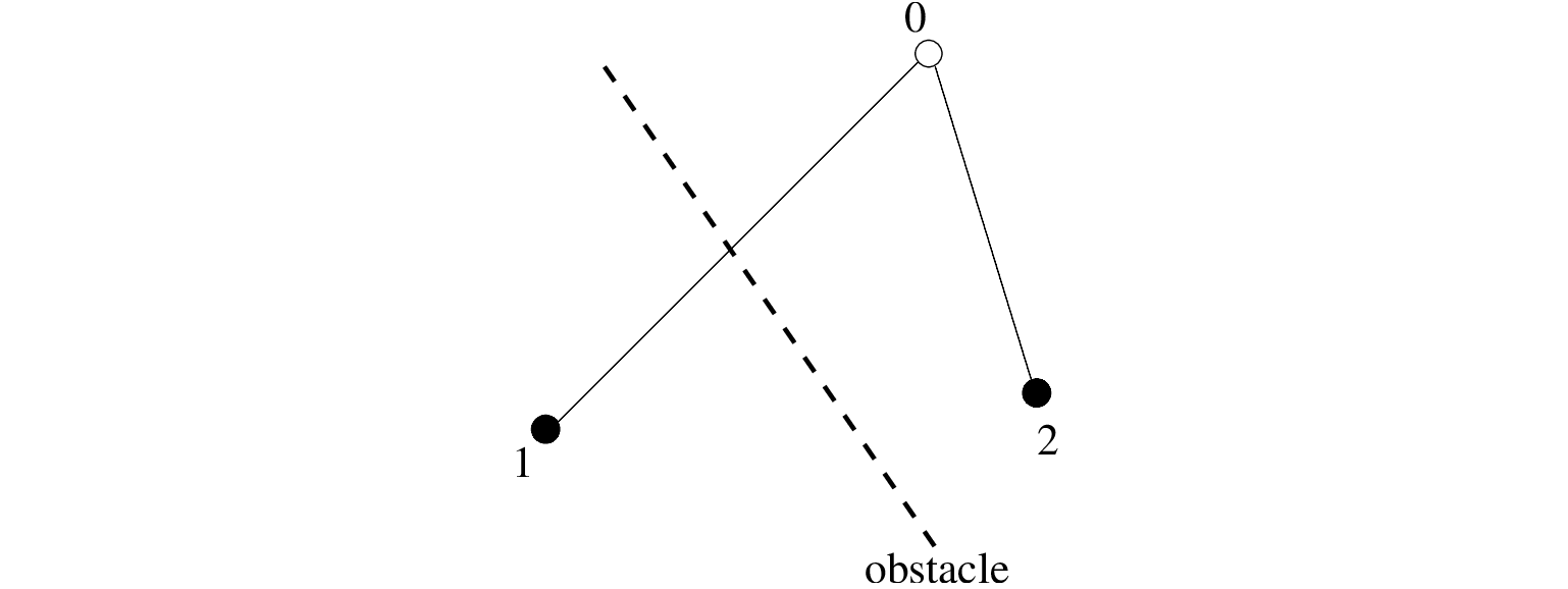the contribution of a neighbouring grid point (point 1 in this case) is reduced by $K_t^2$, if the connection between the two grid points crosses the obstacle. (Note that the power 2 comes from the definition of the transmission coefficient which is in terms of wave height). The contribution from point 2 in the computation of point 0 is not reduced because there is no obstacle crossing in between; the program takes $K_t=1$ for this point.


A consequence of the above procedure is that the results are the same as long as the obstacle crosses the same grid lines. Thus the results for the situation shown would be the same if the obstacle would be longer as long as the end would be in the same mesh. Another consequence is that an obstacle has to cross at least a few grid lines in order to have a noticeable effect, see Figure 3.7.


After the transmission coefficient has been calculated, it is used in the propagation terms of the action balance equation. In curvilinear coordinates, the propagation terms (including time-derivative, but ignoring dependence on $\sigma$ and $\theta$ temporarily) read

$$\left ( \frac{1}{\Delta t} + (D_{x,1} + D_{x,2})c_{x,i,j}^+ + (D_{y,1}+D_{y,2}) c_{y,i,j}^+ \right ) N_{i,j}^+$$

$$- \frac{N_{i,j}^-}{\Delta t} - D_{x,1} (c_x K^2_{t,1} N)_{i-1,j}^+ - D_{y,1} (c_y K^2_{t,1} N)_{i-1,j}^+$$

$$- D_{x,2} (c_x K^2_{t,2} N)_{i,j-1}^+ - D_{y,2} (c_y K^2_{t,2} N)_{i,j-1}^+ = S_{i,j}^+$$ (3.113)

In order to simplify the procedure, a reflected wave in a grid point is calculated from the incident wave components in the same grid point. This introduces numerical inaccuracies, but that is not uncommon in numerical models. A basic condition in numerical models is that the approximation approaches the correct limit as smaller and smaller step sizes are used.


A reflected wave component in the target grid point 0, as illustrated by the arrow pointing away from the obstacle in Figure 3.9,

Figure 3.9: Schematic sketch of reflection in SWAN.

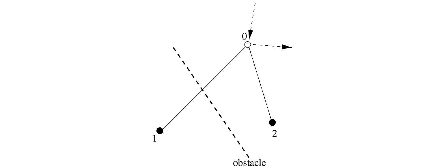would get contributions from grid points 1 and 2 if there would not be an obstacle. If the obstacle is there in the way shown, the contribution from point 2 is unchanged, but the contribution from point 1 is

• reduced by a transmission coefficient and
• partially replaced by the reflection of an incoming component in point 0.

Reflection only works when both grid points 0 and 1, as shown in Figure 3.9, are wet points. This implies that obstacle lines are only effective when bordered by wet points on both sides of the obstacle.