Next: Transformation from relative to Up: Numerical approaches Previous: Crossing of obstacle and

Two methods are considered in SWAN for integration over frequency space. The first method is the common
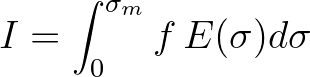
trapezoidal rule. We consider the following integration
 is the highest spectral frequency and
  is an arbitrary function. Usually, this function may be
 ,
,  or
or  with
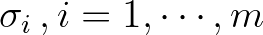
with  a power. We assume a discrete (logarithmic) distribution
of frequencies:
a power. We assume a discrete (logarithmic) distribution
of frequencies:
 .
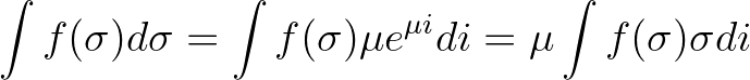
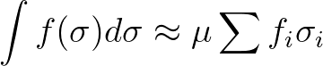
The approximation of (3.117) is as follows
.
The approximation of (3.117) is as follows
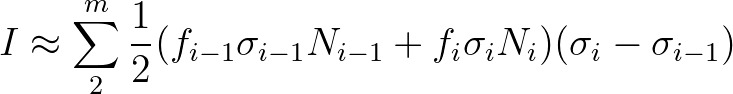 (3.118)
 .
We have,
.
We have,
 (3.119)
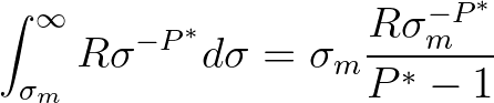
has a tail with power
(3.119)
has a tail with power  , so that
 .
Hence,
.
Hence,
 (3.120)
 .
makes use of the logarithmic discrete distribution of frequencies.
We introduced two variables in SWAN: FRINTF and FRINTH. The first is equal to
.
makes use of the logarithmic discrete distribution of frequencies.
We introduced two variables in SWAN: FRINTF and FRINTH. The first is equal to
 , the latter to
 . Hence,
 with
with
 and can be approximated as
 .
, i.e.
.
, i.e.  is transformed as follows
 (3.121)
 (3.122)
 space are
 and
and
 .
. Furthermore, the discrete integration extends
to
.
. Furthermore, the discrete integration extends
to
 , where
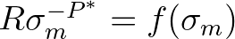
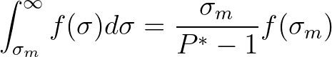
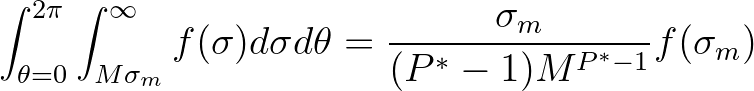
 . Then the contribution by the tail is
 (3.123)
has a tail with power , the integral over has a tail contribution of
(3.123)
has a tail with power , the integral over has a tail contribution of
 (3.124)
 is close to 1, the tail factor can be approximated as
 (3.125)
 FRINTH,
  PWTAIL(1) and
  MSC. The value of
depends on the quantity that is integrated. For instance, in the computation of
MSC. The value of
depends on the quantity that is integrated. For instance, in the computation of  ,
,
 . Note that it is required that , otherwise the integration fails.
The SWAN team 2026-03-13