Next: Write or plot intermediate Up: Output Previous: Output locations Index
For definitions of output parameters, see Appendix A.
WARNING:
When integral parameters are computed by the user from the output spectrum of SWAN, differences with
the SWAN-computed parameters may occur. The reasons are:
          | ..........|
QUANTity <             > 'short' 'long' [lexp] [hexp]  [excv]                   &
          | ..........|

     [power]               (For output quantities PER, RPER and WLEN)           &

     [ref]                 (For output quantity TSEC)                           &

     [fswell]              (For output quantity HSWELL)                         &

     [fmin] [fmax]         (For all integral parameters, like HS, (R)TM01 ...)  &

      |-> PROBLEMcoord |
     <                  >  (For directions (DIR, TDIR, PDIR)
      |   FRAME        |    and vectors (FORCE, WIND, VEL, TRANSP))

With this command the user can influence
| |...| | ||
| < > | the output parameters are the same as given in command BLOCK. | |
| |...| | ||
| `short' | user preferred short name of the output quantity (e.g. the name appearing in | |
| the heading of a table written by SWAN). If this option is not used, SWAN | ||
| will use a realistic name. | ||
| `long' | long name of the output quantity (e.g. the name appearing in the heading of a | |
| block output written by SWAN). If this option is not used, SWAN will use a | ||
| realistic name. | ||
| [lexp] | lowest expected value of the output quantity. | |
| [hexp] | highest expected value of the output quantity; the highest expected value is | |
| used by SWAN to determine the number of decimals in a table with heading. | ||
| So the QUANTITY command can be used in case the default number of decimals | ||
| in a table is unsatisfactory. | ||
| [excv] | in case there is no valid value (e.g. wave height in a dry point) this | |
| exception value of the output quantity is written in a table or block output. |
| [power] | power  appearing in the definition of PER, RPER and WLEN appearing in the definition of PER, RPER and WLEN |
|
| (see Appendix A). Note that the value for [power] given for PER | ||
| affects also the value of RPER; the power for WLEN is independent of that | ||
| of PER or RPER. | ||
| Default: [power]=1. | ||
| [ref] | reference time used for the quantity TSEC. | |
| Default value: starting time of the first computation, except in cases where | ||
| this is later than the time of the earliest input. In these cases, the time of | ||
| the earliest input is used. | ||
| [fswell] | upper limit of frequency range used for computing the quantity HSWELL | |
| (see Appendix A). | ||
| Default: [fswell] = 0.1 Hz. | ||
| [fmin] | lower limit of frequency range used for computing integral parameters. | |
| Default: [fmin] = 0.0 Hz. | ||
| [fmax] | upper limit of frequency range used for computing integral parameters. | |
| Default: [fmax] = 1000.0 Hz (acts as infinity). | ||
| PROBLEMCOORD |  vector components are relative to the vector components are relative to the  and and  axes of the problem axes of the problem |
|
| coordinate system: | ||
 directions are counterclockwise relative to the positive axis of the directions are counterclockwise relative to the positive axis of the |
||
| problem coordinate system if Cartesian direction convention is used (see | ||
| command SET) | ||
| directions are relative to North (clockwise) if Nautical direction |
||
| convention is used (see command SET) | ||
| FRAME | If output is requested on sets created by command FRAME or automatically | |
| (COMPGRID or BOTTGRID): | ||
| vector components are relative to the and axes of the frame |
||
| coordinate system | ||
| directions are counterclockwise relative to the positive axis of the |
||
| frame coordinate system if Cartesian direction convention is used (see | ||
| command SET) | ||
| directions are relative to North (clockwise) if Nautical direction |
||
| convention is used (see command SET) |
Examples:
| QUANTITY Xp hexp=100. | for simulations of lab. experiments | |
| QUANTITY HS TM01 RTMM10 excv=-9. | to change the exception value for  , , |
|
 and relative and relative  |
||
| QUANTITY HS TM02 FSPR fmin=0.03 fmax=0.5 | to compute , 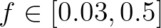 and frequency and frequency |
|
| spreading by means of integration over | ||
![$f \in [0.03, 0.5]$](img147.png) |
||
| QUANTITY Hswell fswell=0.08 | to change the value of [fswell] | |
| QUANTITY Per short='Tm-1,0' power=0. | to redefine average wave period | |
| QUANTITY Transp Force Frame | to obtain vector components and | |
| direction with respect to the frame |
OUTPut OPTIons 'comment' (TABle [field]) (BLOck [ndec] [len]) (SPEC [ndec])
This command enables the user to influence the format of block, table and spectral output.
| comment | a comment character; is used in comment lines in the output | |
| Default: comment = % | ||
| field | length of one data field in a table. Minimum is 8 and maximum is 16. | |
| Default: field = 12 | ||
| ndec | number of decimals in block (if appearing after keyword BLOCK) or | |
| 2D spectral output (if appearing after keyword SPEC). Maximum is 9. | ||
| Default: ndec = 4 (in both block and spectral outputs) | ||
| len | number of data on one line of block output. Maximum is 9999. | |
| Default: len = 6 |
                 | -> HEADer   |
BLOck  'sname'  <               > 'fname' (LAYout [idla])
                 |    NOHEADer |

           | HSign     |
           |           |
           | HSWEll    |
           |           |
           | DIR       |
           |           |
           | PDIR      |
           |           |
           | TDIR      |
           |           |
           | TM01      |
           |           |
           | RTM01     |
           |           |
           | RTP       |
           |           |
           | TPS       |
           |           |
           | PER       |
           |           |
           | RPER      |
           |           |
           | TMM10     |
           |           |
           | RTMM10    |
           |           |
           | TM02      |
           |           |
           | FSPR      |
           |           |
           | DSPR      |
           |           |
           | QP        |
           |           |
           | DEPth     |
           |           |
           | WATLev    |
           |           |
           | BOTLev    |
           |           |
           | VEL       |
           |           |
           | FRCoef    |
           |           |
           | WIND      |
           |           |
           | AICE      |
           |           |
           | HICE      |
           |           |
           | HBIG      |
           |           |
           | PROPAgat  |
           |           |
           | PROPXy    |
           |           |
           | PROPTheta |
           |           |
           | PROPSigma |
           |           |
           | GENErat   |
           |           |
           | GENWind   |
           |           |
           | REDIst    |
           |           |
           | REDQuad   |
           |           |
           | REDTriad  |                                          | -> Sec  |
     <    <             >  [unit] > (OUTput [tbegblk] [deltblk]) <     MIn   >
           | DISSip    |                                          |    HR   |
           |           |                                          |    DAy  |
           | DISBot    |
           |           |
           | DISSUrf   |
           |           |
           | DISWcap   |
           |           |
           | DISSWell  |
           |           |
           | DISVeg    |
           |           |
           | DISMud    |
           |           |
           | DISIce    |
           |           |
           | RADStr    |
           |           |
           | QB        |
           |           |
           | GAMMA     |
           |           |
           | TRAnsp    |
           |           |
           | FORce     |
           |           |
           | UBOT      |
           |           |
           | URMS      |
           |           |
           | TMBOT     |
           |           |
           | WLENgth   |
           |           |
           | LWAVP     |
           |           |
           | STEEpness |
           |           |
           | BFI       |
           |           |
           | NPLants   |
           |           |
           | DHSign    |
           |           |
           | DRTM01    |
           |           |
           | LEAK      |
           |           |
           | TIME      |
           |           |
           | TSEC      |
           |           |
           | XP        |
           |           |
           | YP        |
           |           |
           | DIST      |
           |           |
           | SETUP     |
           |           |
           | PTHSign   |
           |           |
           | PTRTP     |
           |           |
           | PTWLEN    |
           |           |
           | PTDIR     |
           |           |
           | PTDSPR    |
           |           |
           | PTWFRAC   |
           |           |
           | PTSTEEpne |
           |           |
           | PARTITion |
CANNOT BE USED IN 1D-MODE.
With this optional command the user indicates that one or more spatial
distributions should be written to a file.
| 'sname' | name of frame or group (see commands FRAME or GROUP) | |
| HEADER | with this option the user indicates that the output should be written to a file | |
| with header lines. The text of the header indicates run identification (see | ||
| command PROJECT), time, frame name or group name ('sname'), variable and | ||
| unit. The number of header lines is 8. | ||
| Note: the numerical values in the file are in the units indicated in the header. | ||
| NOHEADER | with this option the user indicates that the output should be written to a file | |
| without header lines. | ||
| 'fname' | name of the data file where the output is to be written to. | |
| Default for option HEADER is the PRINT file. In case of NOHEADER the | ||
| filename is required. Below a few remarks on the file formats. | ||
| Basically, the output files generated by SWAN are human-readable files that | ||
| use ASCII character encoding. Such files can be open and edit in any text editor | ||
| or can be viewed in Matlab or Excel. However, if the user specifies the extension | ||
| of the output file as `.mat', a binary MATLAB file will be generated. This file | ||
| requires less space on your computer and can be loaded in MATLAB much faster | ||
| than an ASCII file. Also note that the output parameters are stored as single | ||
| precision. (Hence, use the Matlab command double for conversion to double | ||
| precision, if necessary.) Binary MATLAB files are particularly useful for the | ||
| computation with unstructured grids. A number of MATLAB scripts are provided | ||
| with the SWAN source code that can be used to plot wave parameters as maps | ||
| in a simple way. | ||
| Another option is to write the output to a netCDF format (Network Common | ||
| Data Form). The file extension must be in this case `.nc'. This format is | ||
| self-describing and machine independent. Moreover, it is an open standard and | ||
| portable. This will enhance accessibility of data exchange and also easily | ||
| facilitate using output from one application as input to another. | ||
| Like MATLAB files, storage and retrieval of netCDF files is very fast. | ||
| Since version 41.41, SWAN can generate VTK files that can be viewed in | ||
| Paraview, an open-source, general-purpose visualization package, available for | ||
| Windows, Mac and Linux (see https://www.paraview.org). The basic extension | ||
| is `.vtk', but SWAN will generate various XML-based file formats depending on | ||
| the grid types (*.vts associated with structured grids and *.vtu containing | ||
| unstructured mesh data). Like netCDF files, the VTK XML files are binary, | ||
| self-descriptive (include plain text metadata) and portable (cross-platform). | ||
| In addition, a key benefit is that there is no need to collect VTK files residing | ||
| on separate processes of a distributed memory machine (after execution of | ||
| SWAN in parallel). Paraview can simply visualize the whole domain that | ||
| consists of several subdomains. | ||
| LAY-OUT | with this option the user can prescribe the lay-out of the output to file with | |
| the value of [idla]. | ||
| [idla] | see command READINP (options are: [idla]=1, 3, 4). Option 4 is recommended | |
| for postprocessing an ASCII file by MATLAB, however, in case of a generated | ||
| binary MATLAB file option 3 is recommended. | ||
| Default: [idla] = 1. | ||
| ONLY MEANT FOR STRUCTURED GRIDS. |
For definitions of the output quantities, see Appendix A.
Note that the wave parameters in the output of SWAN are computed from the wave spectrum over the prognostic part of the spectrum
with the diagnostic tail added. Their value may therefore deviate slightly from values computed by the user from the
output spectrum of SWAN which does not contain the diagnostic tail.
| HSIGN | significant wave height (in m). | |
| HSWELL | swell wave height (in m). | |
| DIR | mean wave direction (Cartesian or Nautical convention, see command SET). | |
| For Cartesian convention: relative to axis of the problem coordinate system |
||
| (counterclockwise); possible exception: in the case of output with BLOCK | ||
| command in combination with command FRAME, see command QUANTITY. | ||
| PDIR | peak wave direction in degrees. | |
| For Cartesian convention: relative to axis of the problem coordinate system |
||
| (counterclockwise); possible exception: in the case of output with BLOCK | ||
| command in combination with command FRAME, see command QUANTITY. | ||
| TDIR | direction of energy transport in degrees. | |
| For Cartesian convention: relative to axis of the problem coordinate system |
||
| (counterclockwise); possible exception: in the case of output with BLOCK | ||
| command in combination with command FRAME, see command QUANTITY. | ||
| TM01 | mean absolute wave period (in s). | |
| RTM01 | mean relative wave period (in s). | |
| RTP | peak period (in s) of the variance density spectrum (relative frequency spectrum). | |
| TPS | 'smoothed' peak period (in s). | |
| PER | mean absolute wave period (in s). | |
| RPER | mean relative wave period (in s). | |
| TMM10 | mean absolute wave period (in s). | |
| RTMM10 | mean relative wave period (in s). | |
| TM02 | mean absolute zero-crossing period (in s). | |
| FSPR | the normalized width of the frequency spectrum. | |
| DSPR | directional spreading of the waves (in degrees). | |
| QP | peakedness of the wave spectrum (dimensionless). | |
| DEPTH | water depth (in m) (not the bottom level!). | |
| WATLEV | water level (in m). | |
| Output is in both active and non-active points. | ||
| Note: exception value for water levels must be given! | ||
| (See command INPGRID WLEVEL EXCEPTION). | ||
| BOTLEV | bottom level (in m). | |
| Output is in both active and non-active points. | ||
| Note: exception value for bottom levels must be given! | ||
| (See command INPGRID BOTTOM EXCEPTION). | ||
| VEL | current velocity (vector; in m/s). | |
| Relative to axis of the problem coordinate system (counterclockwise); |
||
| possible exception: in the case of output with BLOCK command | ||
| in combination with command FRAME, see command QUANTITY. | ||
| FRCOEF | friction coefficient (equal to [cfw] or [kn] in command FRICTION). | |
| WIND | wind velocity (vector; in m/s). | |
| Relative to axis of the problem coordinate system (counterclockwise); |
||
| possible exception: in the case of output with BLOCK command | ||
| in combination with command FRAME, see command QUANTITY. | ||
| AICE | ice concentration (as a fraction from 0 to 1). | |
| HICE | ice thickness (in meters). | |
| HBIG | bound ig wave height (in m). | |
| Note: only to be specified for surfbeat (IEM) during first COMPUTE. |
| PROPAGAT | sum of PROPXY, PROPTHETA and PROPSIGMA | |
(in W/m or m/s, depending on command SET). or m/s, depending on command SET). |
||
| PROPXY | energy propagation in geographic space; sum of and direction |
|
| terms (in W/m or m/s, depending on command SET). |
||
| PROPTHETA | energy propagation in theta space | |
| (in W/m or m/s, depending on command SET). |
||
| PROPSIGMA | energy propagation in sigma space | |
| (in W/m or m/s, depending on command SET). |
||
| GENERAT | total energy generation | |
| (in W/m or m/s, depending on command SET). |
||
| GENWIND | energy generation due to wind | |
| (in W/m or m/s, depending on command SET). |
||
| REDIST | total energy redistribution | |
| (in W/m or m/s, depending on command SET). |
||
| REDQUAD | energy redistribution due to quadruplets | |
| (in W/m or m/s, depending on command SET). |
||
| REDTRIAD | energy redistribution due to triads | |
| (in W/m or m/s, depending on command SET). |
||
| DISSIP | total energy dissipation | |
| (in W/m or m/s, depending on command SET). |
||
| DISBOT | energy dissipation due to bottom friction | |
| (in W/m or m/s, depending on command SET). |
||
| DISSURF | energy dissipation due to surf breaking | |
| (in W/m or m/s, depending on command SET). |
||
| DISWCAP | energy dissipation due to whitecapping | |
| (in W/m or m/s, depending on command SET). |
||
| DISSWELL | energy dissipation due to swell dissipation | |
| (in W/m or m/s, depending on command SET). |
||
| DISVEG | energy dissipation due to vegetation | |
| (in W/m or m/s, depending on command SET). |
||
| DISMUD | energy dissipation due to mud | |
| (in W/m or m/s, depending on command SET). |
||
| DISICE | energy dissipation due to sea ice | |
| (in W/m or m/s, depending on command SET). |
||
| RADSTR | energy transfer between waves and currents due to radiation stress | |
| (in W/m or m/s, depending on command SET). |
| QB | fraction of breaking waves due to depth-induced breaking. | |
| GAMMA | breaker index derived from the beta-kd model. | |
| TRANSP | transport of energy (vector; in W/m or m /s, depending on command SET). /s, depending on command SET). |
|
| Relative to axis of the problem coordinate system (counterclockwise); |
||
| possible exception: in the case of output with BLOCK command | ||
| in combination with command FRAME, see command QUANTITY. | ||
| FORCE | wave-induced force per unit surface area (vector; in N/m). |
|
| Relative to axis of the problem coordinate system (counterclockwise); |
||
| possible exception: in the case of output with BLOCK command | ||
| in combination with command FRAME, see command QUANTITY. | ||
| UBOT | the rms-value of the maxima of the orbital velocity near the bottom (in m/s). | |
| Output only if command FRICTION is used. If one wants to output UBOT but | ||
| friction is ignored in the computation, then one should use the command | ||
| FRICTION with the value of the friction set to zero (FRICTION COLLINS 0). | ||
| URMS | the rms-value of the orbital velocity near the bottom (in m/s). | |
| If one wants to output URMS but friction is ignored in the computation, | ||
| then one should use the command FRICTION with the value of the friction | ||
| set to zero (FRICTION COLLINS 0). | ||
| TMBOT | the bottom wave period (in s). | |
| WLEN | average wave length (in m). | |
| LWAVP | peak wave length (in m). | |
| STEEPNESS | average wave steepness (dimensionless). | |
| BFI | Benjamin-Feir index (dimensionless). | |
| NPLANTS | number of plants per square meter. | |
| DHSIGN | the difference in significant wave height as computed in the last two iterations. | |
| This is not the difference between the computed values and the final limit of | ||
| the iteration process, at most an indication of this difference. | ||
| DRTM01 | the difference in average wave period (RTM01) as computed in the last two | |
| iterations. This is not the difference between the computed values and the | ||
| final limit of the iteration process, at most an indication of this difference. | ||
| LEAK | numerical loss of energy equal to
 across boundaries across boundaries |
|
 = [dir1] and = [dir1] and  = [dir2] of a directional sector (see = [dir2] of a directional sector (see |
||
| command CGRID). | ||
| TIME | Full date-time string as part of line used in TABLE only. Useful only in case of | |
| nonstationary computations. | ||
| TSEC | Time in seconds with respect to a reference time (see command QUANTITY). | |
| Useful only in case of nonstationary computations. | ||
| XP | user instructs SWAN to write the coordinate in the problem coordinate system |
|
| of the output location. | ||
| YP | user instructs SWAN to write the coordinate in the problem coordinate system |
|
| of the output location. | ||
| DIST | if output has been requested along a curve (see command CURVE) then the distance | |
| along the curve can be obtained with the command TABLE. DIST is the distance | ||
| along the curve measured from the first point on the curve to the output location | ||
| on the curve in meters (also in the case of spherical coordinates). | ||
| SETUP | Set-up due to waves (in m). | |
| PTHSIGN | user requests partition of the significant wave height (in m). | |
| Partition of wave spectra is based on the watershed algorithm of | ||
| Hanson and Phillips (2001). First partition is due to wind sea and | ||
| the remaining partitions are the swell, from highest to lowest | ||
| significant wave height. There will be at most 10 partitions. | ||
| PTRTP | user requests partition of the relative peak period (in s). | |
| PTWLEN | user requests partition of the average wave length (in m). | |
| PTDIR | user requests partition of the peak wave direction in degrees. | |
| For Cartesian convention: relative to axis of the problem coordinate system |
||
| (counterclockwise); possible exception: in the case of output with BLOCK | ||
| command in combination with command FRAME, see command QUANTITY. | ||
| PTDSPR | user requests partition of the directional spreading (in degrees). | |
| PTWFRAC | user requests partition of the wind fraction (dimensionless). | |
| This indicates the fraction of that partition that is actively being forced | ||
| by the wind. | ||
| PTSTEEP | user requests partition of the wave steepness (dimensionless). | |
| PARTIT | user instructs SWAN to generate the raw spectral partition file meant | |
| for wave system tracking post-processing. | ||
| Details on the file format and meaning of different parameters may be found in | ||
| http://polar.ncep.noaa.gov/waves/workshop/pdfs/ | ||
| WW3-workshop-exercises-day4-wavetracking.pdf. | ||
| Note that this command should not be combined with any other parameters | ||
| in BLOCK, although the following parameters will be automatically included, | ||
| namely: coordinates, depth, wind, current, Hs, Tp, wave direction, directional | ||
| spreading, and wave length. Also note that PARTIT cannot be used as an | ||
| output parameter in TABLE. | ||
| [unit] | this controls the scaling of output. The program divides computed values by [unit] | |
| before writing to file, so the user should multiply the written value by [unit] to | ||
| obtain the proper value. | ||
| Default: if HEADER is selected, value is written as a 5 position integer. | ||
| SWAN takes [unit] such that the largest number occurring in the block | ||
| can be printed. | ||
| If NOHEADER is selected, values are printed in floating-point format, [unit] = 1. | ||
| OUTPUT | the user requests output at various times. If the user does not use this option, the | |
| program will give BLOCK output for the last time step of the computation. | ||
| [tbegblk] | begin time of the first field of the variable, the format is: | |
| 1 : ISO-notation 19870530.153000 | ||
| 2 : (as in HP compiler) '30May87 15:30:00' |
||
| 3 : (as in Lahey compiler) 05/30/87.15:30:00 | ||
| 4 : 15:30:00 | ||
| 5 : 87/05/30 15:30:00' | ||
| 6 : as in WAM 8705301530 | ||
| This format is installation dependent. See Implementation Manual or ask the | ||
| person who installed SWAN on your computer. Default is ISO-notation. | ||
| [deltblk] | time interval between fields, the unit is indicated in the next option: | |
| SEC unit seconds | ||
| MIN unit minutes | ||
| HR unit hours | ||
| DAY unit days |
                 | -> HEADer   |
                 |             |
TABle  'sname'  <     NOHEADer  >  'fname'                                 &
                 |             |
                 |    INDexed  |

             | ...      |                                     | -> Sec  |
       <    <             >   > (OUTput [tbegtbl] [delttbl]  <     MIn   >)
             | ...      |                                     |    HR   |
                                                              |    DAy  |
With this optional command the user indicates that for each location of the output location set 'sname' (see commands POINTS, CURVE, FRAME or GROUP) one or more variables should be written to a file. The keywords HEADER and NOHEADER determine the appearance of the table; the filename determines the destination of the data.
| 'sname' | name of the set of POINTS, CURVE, FRAME or GROUP | |
| HEADer | output is written in fixed format to file with headers giving name of variable | |
| and unit per column. A disadvantage of this option is that the data are written | ||
| in fixed format; numbers too large to be written will be shown as: ****. | ||
| Number of header lines is 4. | ||
| NOHEADer | output is written in floating point format to file and has no headers; it is | |
| intended primarily for processing by other programs. With some spreadsheet | ||
| programs, however, the HEADER option works better. | ||
| INDexed | a table on file is produced which can be used directly (without editing) as input | |
| to ARCVIEW, ARCINFO, etc. The user should give two TABLE commands, one | ||
| to produce one file with XP and YP as output quantities, the other with HS, RTM01 | ||
| or other output quantities, such as one wishes to process in ARCVIEW | ||
| or ARCINFO. The first column of each file produced by SWAN with this command | ||
| is the sequence number of the output point. The last line of each file is | ||
| the word END. | ||
| 'fname' | name of the data file where the output is to be written to. | |
| Default for option HEADER is output to the PRINT file. In case of NOHEADER the | ||
| filename is required. | ||
| |...| | ||
| < > | the output parameters are the same as given in command BLOCK. | |
| |...| | ||
| OUTPUT | the user requests output at various times. If the user does not use this option, | |
| the program will give TABLE output for the last time step of the computation. | ||
| [tbegtbl] | begin time of the first field of the variable, the format is: | |
| 1 : ISO-notation 19870530.153000 | ||
| 2 : (as in HP compiler) '30May87 15:30:00' |
||
| 3 : (as in Lahey compiler) 05/30/87.15:30:00 | ||
| 4 : 15:30:00 | ||
| 5 : 87/05/30 15:30:00' | ||
| 6 : as in WAM 8705301530 | ||
| This format is installation dependent. See Implementation Manual or ask the | ||
| person who installed SWAN on your computer. Default is ISO-notation. | ||
| [delttbl] | time interval between fields, the unit is indicated in the next option: | |
| SEC unit seconds | ||
| MIN unit minutes | ||
| HR unit hours | ||
| DAY unit days |
Unless specifying (see command BLOCK), the and components of the vectorial quantities VEL,
FORCE and TRANSPORT are always given with respect to the problem coordinate system.
The number of decimals in the table varies for the output parameters; it depends on the value of [hexp], given
in the command QUANTITY.
                  |    SPEC1D |    | -> ABSolute |    | -> S |
SPECout  'sname' <             >  <               >  <        >  'fname' &
                  | -> SPEC2D |    |    RELative |    |    L |

                                      | -> Sec  |
         OUTput [tbegspc] [deltspc]  <     MIn   >
                                      |    HR   |
                                      |    DAy  |
With this optional command the user indicates that for each location of the output location set 'sname' (see commands POINTS, CURVE, FRAME or GROUP) the 1D or 2D variance / energy (see command SET) density spectrum (either the relative frequency or the absolute frequency spectrum) is to be written to a data file. The name 'fname' is required in this command.
| 'sname' | name of the set of POINTS, CURVE, FRAME or GROUP | |
| SPEC2D | means that 2D (frequency-direction) spectra are written to file according to the | |
| format described in Appendix D. Note that this output file can be used for | ||
| defining boundary conditions for subsequent SWAN runs (command BOUNDSPEC). | ||
| SPEC1D | means that 1D (frequency) spectra are written to file according to the format | |
| described in Appendix D. Note that this output file can be used for defining | ||
| boundary conditions for subsequent SWAN runs (command BOUNDSPEC). | ||
| ABS | means that spectra are computed as function of absolute frequency (i.e. the | |
| frequency as measured in a fixed point). | ||
| REL | means that spectra are computed as function of relative frequency (i.e. the | |
| frequency as measured when moving with the current). | ||
| S | frequencies above the infragravity frequency cut-off  are taken into account. are taken into account. |
|
| Note: only relevant for surfbeat (IEM) modelling. | ||
| L | frequencies below the infragravity frequency cut-off are taken into account. |
|
| Note: only relevant for surfbeat (IEM) modelling. | ||
| 'fname' | name of the data file where the output is written to. | |
| When the extension is `.nc', a netCDF file will be generated automatically. | ||
| OUTPUT | the user requests output at various times. If the user does not use this option, | |
| the program will give SPECOUT output for the last time step of the computation. | ||
| [tbegspc] | begin time of the first field of the variable, the format is: | |
| 1 : ISO-notation 19870530.153000 | ||
| 2 : (as in HP compiler) '30May87 15:30:00' |
||
| 3 : (as in Lahey compiler) 05/30/87.15:30:00 | ||
| 4 : 15:30:00 | ||
| 5 : 87/05/30 15:30:00' | ||
| 6 : as in WAM 8705301530 | ||
| This format is installation dependent. See Implementation Manual or ask the | ||
| person who installed SWAN on your computer. Default is ISO-notation. | ||
| [deltspc] | time interval between fields, the unit is indicated in the next option: | |
| SEC unit seconds | ||
| MIN unit minutes | ||
| HR unit hours | ||
| DAY unit days |
                                                    | -> Sec  |
NESTout 'sname' 'fname' OUTput [tbegnst] [deltnst] <     MIn   >
                                                    |    HR   |
                                                    |    DAy  |
CANNOT BE USED IN 1D-MODE
With this optional command the user indicates that the 2D spectra along a nest boundary 'sname' (see
command NGRID) should be written to a data file with name 'fname'. This name is required in this command.
| 'sname' | name of the set of output locations, as defined in a command NGRID | |
| 'fname' | name of the data file where the output is written to. The file is structured | |
| according to the description in Appendix D, i.e. also the information about the | ||
| location of the boundary are written to this file. SWAN will use this as a check | ||
| for the subsequent nested run. | ||
| OUTPUT | the user requests output at various times. If the user does not use this option, | |
| the program will give NESTOUT output for the last time step of the computation. | ||
| [tbegnst] | begin time of the first field of the variable, the format is: | |
| 1 : ISO-notation 19870530.153000 | ||
| 2 : (as in HP compiler) '30May87 15:30:00' |
||
| 3 : (as in Lahey compiler) 05/30/87.15:30:00 | ||
| 4 : 15:30:00 | ||
| 5 : 87/05/30 15:30:00' | ||
| 6 : as in WAM 8705301530 | ||
| This format is installation dependent. See Implementation Manual or ask the | ||
| person who installed SWAN on your computer. Default is ISO-notation. | ||
| [deltnst] | time interval between fields, the unit is indicated in the next option: | |
| SEC unit seconds | ||
| MIN unit minutes | ||
| HR unit hours | ||
| DAY unit days |
The SWAN team 2026-03-13