Next: Wave-induced set-up Up: Modelling of obstacles Previous: Freeboard dependent reflection and
To accommodate wave diffraction in SWAN simulations, a phase-decoupled refraction-diffraction approximation
is suggested (Holthuijsen et al., 2003). It is expressed in terms of the directional turning rate
of the individual wave components in the 2D wave spectrum. The approximation is based on the mild-slope
equation for refraction and diffraction, omitting phase information. This approach is thus consistent with
the assumption of a quasi-homogeneous wave field. However,
see Section 2.7 for the discussion of the inclusion of wave statistics of inhomogeneous wave
fields due to diffraction.
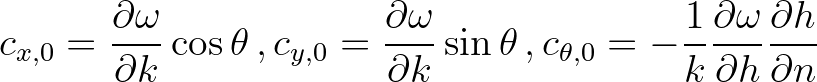
In a simplest case, we assume there are no currents. This means that  . Let denotes the
propagation velocities in geographic and spectral spaces for the situation without diffraction as
. Let denotes the
propagation velocities in geographic and spectral spaces for the situation without diffraction as
 ,
,  and
and  . These are given by
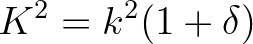
 is the wave number and
  is perpendicular to the wave ray. We consider the following eikonal
equation
is perpendicular to the wave ray. We consider the following eikonal
equation
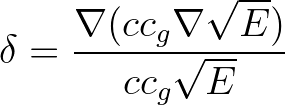
 denoting the diffraction parameter as given by
 is the total energy of the wave field (
 ).
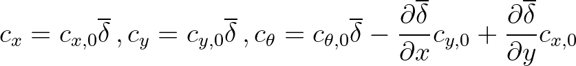
Due to diffraction, the propagation velocities are given by
).
Due to diffraction, the propagation velocities are given by
 in
in  direction. These unduly affected the estimations of the gradients that were
needed to compute the diffraction parameter . The wave field was therefore smoothed with the following
convolution filter:
direction. These unduly affected the estimations of the gradients that were
needed to compute the diffraction parameter . The wave field was therefore smoothed with the following
convolution filter:
![$\displaystyle E_{i,j}^n = E_{i,j}^{n-1} - 0.2 [E_{i-1,j}+E_{i,j-1}-4E_{i,j}+E_{i+1,j}+E_{i,j+1}]^{n-1}
$](img661.png) (2.183)
(2.183)
 is a grid point and the superscript indicates iteration number of the convolution cycle.
The width of this filter (standard deviation) in direction
is a grid point and the superscript indicates iteration number of the convolution cycle.
The width of this filter (standard deviation) in direction  , when applied times is
 (2.184)
 is found to be an optimum value (corresponding to spatial resolution of
1/5 to 1/10 of the wavelength), so that
is found to be an optimum value (corresponding to spatial resolution of
1/5 to 1/10 of the wavelength), so that
 . For the
  direction, the expressions
are identical, with
direction, the expressions
are identical, with  replacing
  . Note that this smoothing is only applied to compute the diffraction
parameter . For all other computations the wave field is not smoothed.
. Note that this smoothing is only applied to compute the diffraction
parameter . For all other computations the wave field is not smoothed.
The SWAN team 2026-03-13