Next: Evolution equation for the Up: Quasi-coherent modelling Previous: Quasi-coherent modelling
The principle result of this section is to present the Wigner distribution which can be viewed as an extension to the variance density spectrum
in the sense that cross-correlation contributions between non-collinear wave components in the wave field are included. Such a field thus
deviates from homogeneous statistics. We begin with a short review of the spectral description of quasi-homogeneous wave fields
and then consider the extension to inhomogeneous fields.
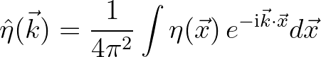
We consider the random sea surface  that is Gaussian distributed with a zero mean. Its Fourier transform is given
by2.4
that is Gaussian distributed with a zero mean. Its Fourier transform is given
by2.4
 (2.188)
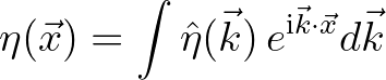
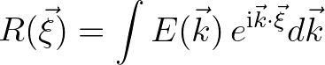
 is the wave number vector. The inverse of this Fourier transform reads
 (2.189)
 and
and  forms the conjugate pair.
 (2.190)
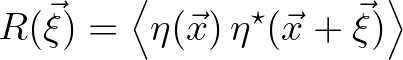
 the separation distance and
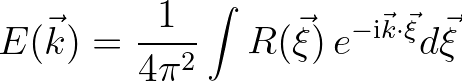
  denoting the complex conjugate. The variance density spectrum is given by
 (2.191)
 (2.192)
 (2.193)
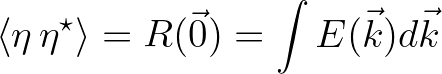
 yields the distribution of variance among different wave numbers.
The first order statistics of the wave field are then completely defined by this spectrum.
yields the distribution of variance among different wave numbers.
The first order statistics of the wave field are then completely defined by this spectrum.
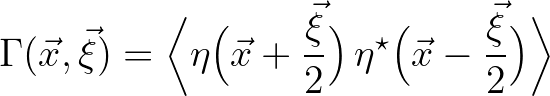
 of surface elevation between
two spatial points
of surface elevation between
two spatial points
 and
and
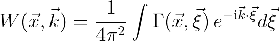
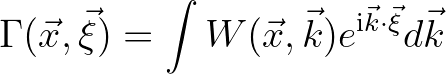
 , called the Wigner distribution,
is symmetric with respect to the spatial lag , so that
, called the Wigner distribution,
is symmetric with respect to the spatial lag , so that
 , and hence
 is a real-valued function.
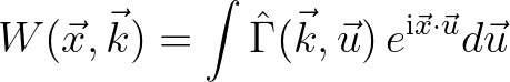
Furthermore, it can also be expressed in terms of the spectrum as follows (Bastiaans, 1979)
is a real-valued function.
Furthermore, it can also be expressed in terms of the spectrum as follows (Bastiaans, 1979)
 (2.196)
 (2.197)
 and
and
 are the mean and difference of two interacting wave components, respectively.
 (2.198)
 (2.199)
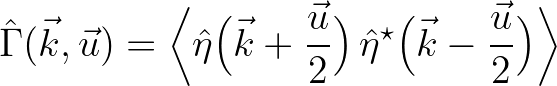
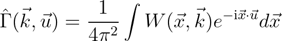
essentially describes the complete second order wave statistics, including the cross-variance contributions, by
virtue of the separation in the wave number
(2.199)
essentially describes the complete second order wave statistics, including the cross-variance contributions, by
virtue of the separation in the wave number  . Furthermore, the local wave variance can be expressed as
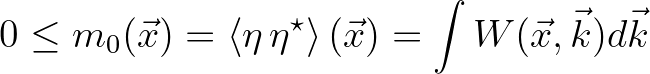 (2.200)
The SWAN team 2026-03-13