Next: Conservative elimination of negative Up: Discretization Previous: Note on the choice
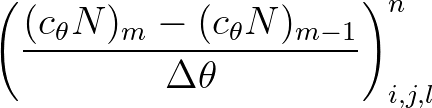
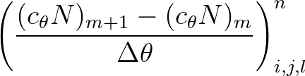
The fluxes in the spectral space
 , as given in Eq. (3.2), should not be approximated
with the first order upwind scheme since, it turns out to be very diffusive for frequencies near the blocking
frequency3.2. Central differences
should be used because of second order accuracy. However, such schemes tend to produce unphysical oscillations
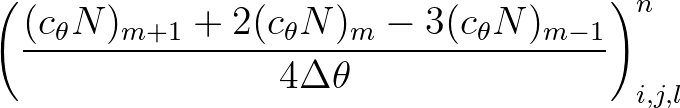
due to relatively large gradients in action density near the blocking frequency. Instead, a hybrid
central/upwind scheme is employed:
, as given in Eq. (3.2), should not be approximated
with the first order upwind scheme since, it turns out to be very diffusive for frequencies near the blocking
frequency3.2. Central differences
should be used because of second order accuracy. However, such schemes tend to produce unphysical oscillations
due to relatively large gradients in action density near the blocking frequency. Instead, a hybrid
central/upwind scheme is employed:
 and
and  are still to be chosen. For all values
 ![$\mu \in [0,1]$](img894.png) and
and ![$\nu \in [0,1]$](img895.png) ,
a blended form arises between first order upwind differencing (
,
a blended form arises between first order upwind differencing ( ) and central differencing
(
) and central differencing
( ). Like the fluxes in the geographical space, both fluxes at
  and
and  acts together with the same sign of
  . The same holds for fluxes at
  and
and  acting together with the same sign of
  . Note that the above scheme is flux conservative and thus suitable
for cases with rapidly varying bathymetry.
. Note that the above scheme is flux conservative and thus suitable
for cases with rapidly varying bathymetry.
 ) yields
(keep in mind that bin
) yields
(keep in mind that bin  is the bin of consideration for the approximation of this refraction term)
 (3.22)
 and
and
 , first order upwinding (
 ) returns
 (3.23)
 and
and
 , we have
 (3.24)
 as one single quantity defined in
directional bins only. Suppose that the divergence of this flux is zero. Applying the above upwind
approximations implies that the wave action flux is constant in every directional bin. Hence, this upwind
scheme () preserves exactly the constancy of this flux. This is called pointwise conservation.
Note that this scheme also preserves causality.
Although the central difference scheme () is flux conservative, it is not pointwise conservative.
Furthermore, due to the nature of this approximation a checkerboard problem may arise. Therefore,
in practice, we always choose
as one single quantity defined in
directional bins only. Suppose that the divergence of this flux is zero. Applying the above upwind
approximations implies that the wave action flux is constant in every directional bin. Hence, this upwind
scheme () preserves exactly the constancy of this flux. This is called pointwise conservation.
Note that this scheme also preserves causality.
Although the central difference scheme () is flux conservative, it is not pointwise conservative.
Furthermore, due to the nature of this approximation a checkerboard problem may arise. Therefore,
in practice, we always choose
 in SWAN.
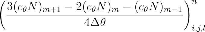
 . This approximation contains three consecutive transport velocities which can either be positive or negative. In other cases,
they are negligibly small (zero crossing), for which central differences () will then be applied (no clear wave direction).
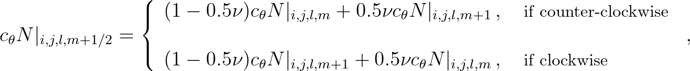
We first consider the counter-clockwise case
. This approximation contains three consecutive transport velocities which can either be positive or negative. In other cases,
they are negligibly small (zero crossing), for which central differences () will then be applied (no clear wave direction).
We first consider the counter-clockwise case
 ,
,
 and
and
 , and the associated approximation then reads
 (3.25)
and
(3.25)
and  are receiving energy from the bin
  . However, bin receives
less energy than bin . Hence, it slows down the turning of the waves.
Since the downstream bin receives some energy, this scheme violates causality. Furthermore, although this scheme is flux conservative, it is
not pointwise conservative, i.e. the energy flux may not remain constant in each directional bin.
The other case is the clockwise one, i.e.
. However, bin receives
less energy than bin . Hence, it slows down the turning of the waves.
Since the downstream bin receives some energy, this scheme violates causality. Furthermore, although this scheme is flux conservative, it is
not pointwise conservative, i.e. the energy flux may not remain constant in each directional bin.
The other case is the clockwise one, i.e.
 ,
,
 and
and
 . For this case, the approximation is given
by
. For this case, the approximation is given
by
 (3.26)
The SWAN team 2026-03-13