Next: Discretization in geographical space Up: Numerical approaches Previous: Introduction
Discretization of Eq. (2.19) is carried out using the finite difference method.
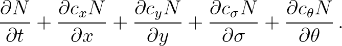
The homogeneous part of Eq. (2.19) is given by
 and
and  in
in  and
and  direction,
respectively. The spectral space is divided into elementary bins with a constant directional
resolution
direction,
respectively. The spectral space is divided into elementary bins with a constant directional
resolution  and a constant relative frequency resolution
 (resulting in a logarithmic frequency distribution). We denote the grid counters as
 ,
,
 ,
,
 and
and
 in , ,
  and
and  spaces, respectively. All variables, including e.g. wave number, group velocity, ambient current
and propagation velocities, are located at points
spaces, respectively. All variables, including e.g. wave number, group velocity, ambient current
and propagation velocities, are located at points  . Time discretization
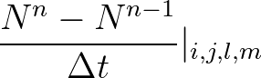
takes place with the implicit Euler technique. We obtain the following approximation of Eq. (3.1):
. Time discretization
takes place with the implicit Euler technique. We obtain the following approximation of Eq. (3.1):
 is a time-level with
  a time step. In case of a stationary computation, the first
term of Eq. (3.2) is removed and denotes an iteration level.
Note that locations in between consecutive counters are reflected with the half-indices.
a time step. In case of a stationary computation, the first
term of Eq. (3.2) is removed and denotes an iteration level.
Note that locations in between consecutive counters are reflected with the half-indices.

![$\displaystyle \frac{[c_x N]_{i+1/2}-[c_x N]_{i-1/2}}{\Delta x}\vert^{n}_{j,l,m} +$](img843.png)
![$\displaystyle \frac{[c_y N]_{j+1/2}-[c_y N]_{j-1/2}}{\Delta y}\vert^{n}_{i,l,m} +$](img844.png)
![$\displaystyle \frac{[c_\sigma N]_{l+1/2}-[c_\sigma N]_{l-1/2}}{\Delta \sigma}\vert^{n}_{i,j,m} +$](img845.png)
![$\displaystyle \frac{[c_\theta N]_{m+1/2}-[c_\theta N]_{m-1/2}}{\Delta \theta}\vert^{n}_{i,j,l}\, ,$](img846.png)