Next: On the approximation of Up: Action density limiter and Previous: Introduction
As explained in Section 3.7.1,
many time scales are involved in the evolution of wind waves. The high-frequency waves have much shorter
time scales than the low-frequency waves, rendering the system of equations
(3.35) stiff. If no special measures are taken,
the need to resolve high-frequency waves at very short time scales would result in extreme computational time. For economy,
it is desirable that a numerical technique can be used with a large, fixed time step. Moreover, we are
mainly interested in the evolution of slowly changing low-frequency waves. For stationary problems,
we are interested in obtaining the steady-state solution.
Unfortunately, the convergence to the steady state is dominated by the
smallest time scale and, in the absence of remedial measures, destabilizing
over- and undershoots will prevent
solution from converging monotonically during the iteration process.
These oscillations arise because of the off-diagonal terms in matrix  ,
which can be dominant over the main diagonal, particularly when the ratio
,
which can be dominant over the main diagonal, particularly when the ratio
 is substantially larger than one. As a consequence,
convergence is slowed down and divergence often occurs.
To accelerate the iteration process without generating instabilities, appropriately small updates must be made
to the level of action density.
is substantially larger than one. As a consequence,
convergence is slowed down and divergence often occurs.
To accelerate the iteration process without generating instabilities, appropriately small updates must be made
to the level of action density.
With the development of the WAM model, a so-called action density limiter was introduced as a remedy to the abovementioned
problem. This action limiter restricts the net growth or
decay of action density to a maximum change at each geographic grid point and spectral bin per time step.
This maximum change corresponds to a fraction of the
omni-directional Phillips equilibrium level (Hersbach and Janssen, 1999).
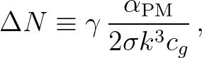
In the context of SWAN (Booij et al., 1999), this is
 denotes the limitation factor,
  is the wave number and
 is the Phillips constant for a Pierson-Moskowitz spectrum
(Komen et al., 1994). Usually,
is the Phillips constant for a Pierson-Moskowitz spectrum
(Komen et al., 1994). Usually,  (Tolman,
1992)3.5.
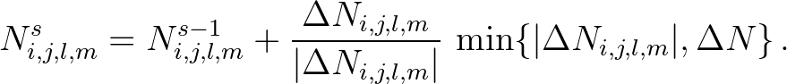
Note that when the physical wind formulation of Janssen (1989,1991a) is applied in SWAN, the original
limiter of Hersbach and Janssen (1999) is employed. Denoting the
total change in
(Tolman,
1992)3.5.
Note that when the physical wind formulation of Janssen (1989,1991a) is applied in SWAN, the original
limiter of Hersbach and Janssen (1999) is employed. Denoting the
total change in  from one iteration to the next after Eq. (3.2) by
 , the action density at the new iteration level is given by
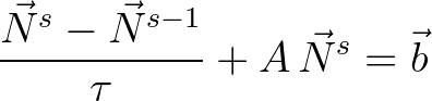
and thus stabilize the iteration process. The system of equations
(3.35) is replaced by the following, iteration-dependent system
, the action density at the new iteration level is given by
and thus stabilize the iteration process. The system of equations
(3.35) is replaced by the following, iteration-dependent system
 a pseudo time step.
The first term of Eq. (3.44) controls the rate of
convergence of the iteration process in the sense that
smaller updates are made due to decreasing , usually
at the cost of increased computational time.
To deal with decreasing time scales at
increasing wave frequency, the amount of under-relaxation is enlarged in
proportion to frequency. This allows a decrease in the computational cost of
under-relaxation, because at lower frequencies larger updates are made. This
frequency-dependent under-relaxation can be achieved by setting
a pseudo time step.
The first term of Eq. (3.44) controls the rate of
convergence of the iteration process in the sense that
smaller updates are made due to decreasing , usually
at the cost of increased computational time.
To deal with decreasing time scales at
increasing wave frequency, the amount of under-relaxation is enlarged in
proportion to frequency. This allows a decrease in the computational cost of
under-relaxation, because at lower frequencies larger updates are made. This
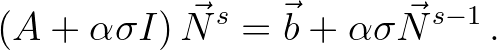
frequency-dependent under-relaxation can be achieved by setting
 ,
where
,
where  is a dimensionless parameter.
The parameter will play an important role in
determining the convergence rate and stability of the iteration process.
Substitution in Eq. (3.44) gives
is a dimensionless parameter.
The parameter will play an important role in
determining the convergence rate and stability of the iteration process.
Substitution in Eq. (3.44) gives
 ), system (3.45) solves
 since,
 is a fixed point of (3.45).
must be determined empirically and thus robustness is impaired.
For increasing values of , the change in action density per iteration will decrease in
the whole spectrum. The consequence of this is twofold. Firstly, it allows a much broader frequency
range in which the action balance equation (3.2) is actually solved without distorting convergence
properties.
Secondly, the use of the limiter will be reduced because more density changes will not exceed the maximum
change due to Eq. (3.42). Clearly, this effect may be augmented by
increasing the value of
is a fixed point of (3.45).
must be determined empirically and thus robustness is impaired.
For increasing values of , the change in action density per iteration will decrease in
the whole spectrum. The consequence of this is twofold. Firstly, it allows a much broader frequency
range in which the action balance equation (3.2) is actually solved without distorting convergence
properties.
Secondly, the use of the limiter will be reduced because more density changes will not exceed the maximum
change due to Eq. (3.42). Clearly, this effect may be augmented by
increasing the value of  in Eq. (3.42).
 ) during the first iteration. Whereas this measure is important
in achieving fast convergence, it does not affect stability, since the
second-generation formulations do not require stabilization.
) during the first iteration. Whereas this measure is important
in achieving fast convergence, it does not affect stability, since the
second-generation formulations do not require stabilization.
The SWAN team 2026-03-13