Next: Implementation of DIA within Up: Numerical approaches Previous: Iteration process and stopping
In the absence of a current, the direction of propagation of the wave crest is equal to that of the wave
energy. For this case, the propagation velocity of energy ( ,
,  ) is equal
to the group velocity (
) is equal
to the group velocity ( ,
,  ). In presence of a current this is not the case, since the propagation
velocities and of energy are changed by the current. Considering the applied numerical procedure
in SWAN, it is initially more convenient to explain the basic principles of the numerical procedure in
the absence of a current than in the situation where a current is present. So, first, we shall focus on
the sweeping technique in the absence of a current. After this, we shall discuss the numerical
procedure in case a current is present.
). In presence of a current this is not the case, since the propagation
velocities and of energy are changed by the current. Considering the applied numerical procedure
in SWAN, it is initially more convenient to explain the basic principles of the numerical procedure in
the absence of a current than in the situation where a current is present. So, first, we shall focus on
the sweeping technique in the absence of a current. After this, we shall discuss the numerical
procedure in case a current is present.
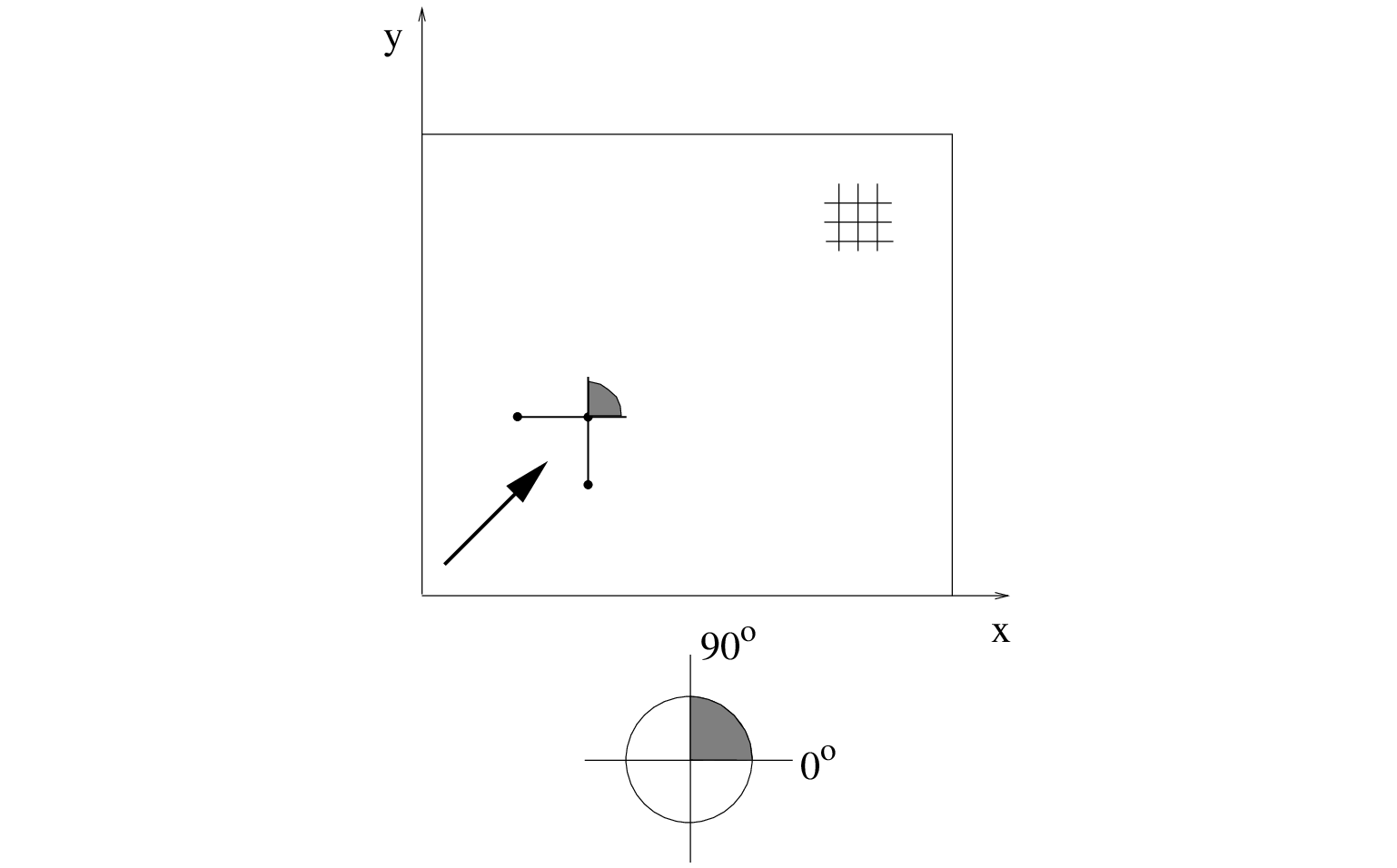
The computational region is a rectangle covered with a rectangular grid. One of the axes (say
the  axis) is chosen arbitrary, for instance perpendicular to the coast.
The state in a grid point (
axis) is chosen arbitrary, for instance perpendicular to the coast.
The state in a grid point ( ,
, ) in an upwind stencil is determined by its up-wave grid points
(
) in an upwind stencil is determined by its up-wave grid points
( ,) and (,
 ). This stencil covers
the propagation of action density within a sector of 0
). This stencil covers
the propagation of action density within a sector of 0 90
90 , in the entire geographic space; see Figure 3.2.
 |
, the next quadrant 90180 is propagated. Rotating the stencil twice more ensures propagation over
all four quadrants (see Figure 3.1). This allows waves to propagate from all directions. Hence, the method
is characterized as a four-sweep technique.
 and the directional interval of each sweep
equals 360
and the directional interval of each sweep
equals 360 . It is expected that the number of iterations may reduced, since the solution is guaranteed to be
updated for all wave directions at all grid points in one series of sweeps, provided the directional interval is
sufficiently small (e.g. 8 sweeps with an interval of 45 each, or 12 sweeps of each 30). This is certainly
the case at deep water where wave rays are just straight lines. However, at shallow water, this becomes less
obvious because of the presence of refraction. In this case the wave energy may jump multiple directional bins in one
(large) time or distance step. It may leave a sweep sector too early or it may even skip this sweep,
especially when the sweep interval is relatively small (
. It is expected that the number of iterations may reduced, since the solution is guaranteed to be
updated for all wave directions at all grid points in one series of sweeps, provided the directional interval is
sufficiently small (e.g. 8 sweeps with an interval of 45 each, or 12 sweeps of each 30). This is certainly
the case at deep water where wave rays are just straight lines. However, at shallow water, this becomes less
obvious because of the presence of refraction. In this case the wave energy may jump multiple directional bins in one
(large) time or distance step. It may leave a sweep sector too early or it may even skip this sweep,
especially when the sweep interval is relatively small ( 30) and depth changes per grid cell are relatively large.
The result is that wave rays erroneously cross and that a number of wave components in one sweep within one time/distance step
overtakes some other bins in another sweep ahead, which implies that causality is violated, resulting in a possible model instability.
See also Section 3.8.3. Hence, for such shallow water cases, choosing a relative large number of
sweeps,
30) and depth changes per grid cell are relatively large.
The result is that wave rays erroneously cross and that a number of wave components in one sweep within one time/distance step
overtakes some other bins in another sweep ahead, which implies that causality is violated, resulting in a possible model instability.
See also Section 3.8.3. Hence, for such shallow water cases, choosing a relative large number of
sweeps,  , is more likely to prove counter-productive.
 ,
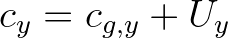
, ) is present. The
main difference is that the propagation velocities of energy are no longer equal to the group velocity
of the waves but become equal to
) is present. The
main difference is that the propagation velocities of energy are no longer equal to the group velocity
of the waves but become equal to
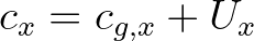 and
and
 . To ensure an unconditionally
stable propagation of action in geographical space in the presence of any current, it is first determined
which spectral wave components of the spectrum can be propagated in one sweep. This implies that all wave
components with
. To ensure an unconditionally
stable propagation of action in geographical space in the presence of any current, it is first determined
which spectral wave components of the spectrum can be propagated in one sweep. This implies that all wave
components with  and
and  are propagated in the first sweep, components with
  and
in the second sweep, components with and
and
in the second sweep, components with and  in the third sweep, and finally, components
and in the fourth sweep.
Since the group velocity of the waves decreases with increasing frequency, the higher frequencies
are more influenced by the current. As a result, the sector boundaries in directional space for these
higher frequencies change more compared to the sector boundaries for the lower frequencies. In general,
four possible configurations do occur (see Figure 3.3). Consider, for instance, one fixed frequency
propagating on a uniform current. The current propagates at an angle of 45 with the axis. The sign
of the current vector and strength of the current are arbitrary. The shaded sectors in Figure 3.3
indicate that all the wave components that are propagating in the direction within the shaded sector, are
propagated in the first sweep (, ).
in the third sweep, and finally, components
and in the fourth sweep.
Since the group velocity of the waves decreases with increasing frequency, the higher frequencies
are more influenced by the current. As a result, the sector boundaries in directional space for these
higher frequencies change more compared to the sector boundaries for the lower frequencies. In general,
four possible configurations do occur (see Figure 3.3). Consider, for instance, one fixed frequency
propagating on a uniform current. The current propagates at an angle of 45 with the axis. The sign
of the current vector and strength of the current are arbitrary. The shaded sectors in Figure 3.3
indicate that all the wave components that are propagating in the direction within the shaded sector, are
propagated in the first sweep (, ).
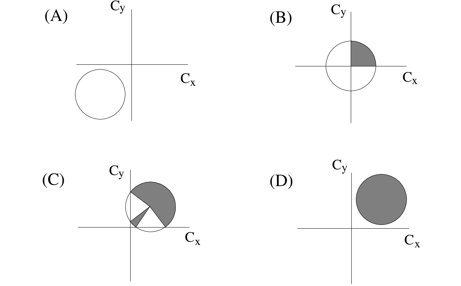 |
and are negative due to a strong
opposing current, i.e. wave blocking occurs. None of the wave components is propagated within the first
sweep. The top-right panel (B) represents a situation in which the current velocity is rather small.
The sector boundaries in directional space are hardly changed by the current such that the sector
boundaries are approximately the same as in the absence of a current. The bottom-left panel (C)
reflects a following current that causes the propagation velocities of the wave components in two
sectors to be larger than zero. In this specific case, all the waves of the shaded sectors are propagated
within the first sweep. The bottom-right panel (D) represents a case with a strong following current
for which all the action is take along with the current. For this case the fully 360 sector is
propagated in the first sweep.