Next: A historical overview of Up: On the approximation of Previous: Energy transport along wave
In this section we discuss how refraction affects the accuracy of the discretization of the total derivative of wave energy along a non-curved wave ray.
Initially, the energy is uniformly distributed over the wave directions.
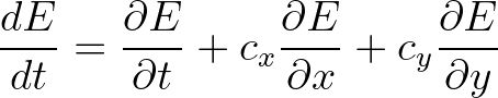
Under these conditions, we reconsider Eq. (3.47),
 (3.54)
 the propagation velocity vector in the geographical space.
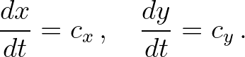
This total derivative indicates that the time rate of change in energy is computed along the wave characteristics defined by the following ODEs
the propagation velocity vector in the geographical space.
This total derivative indicates that the time rate of change in energy is computed along the wave characteristics defined by the following ODEs
 (3.56)
 and
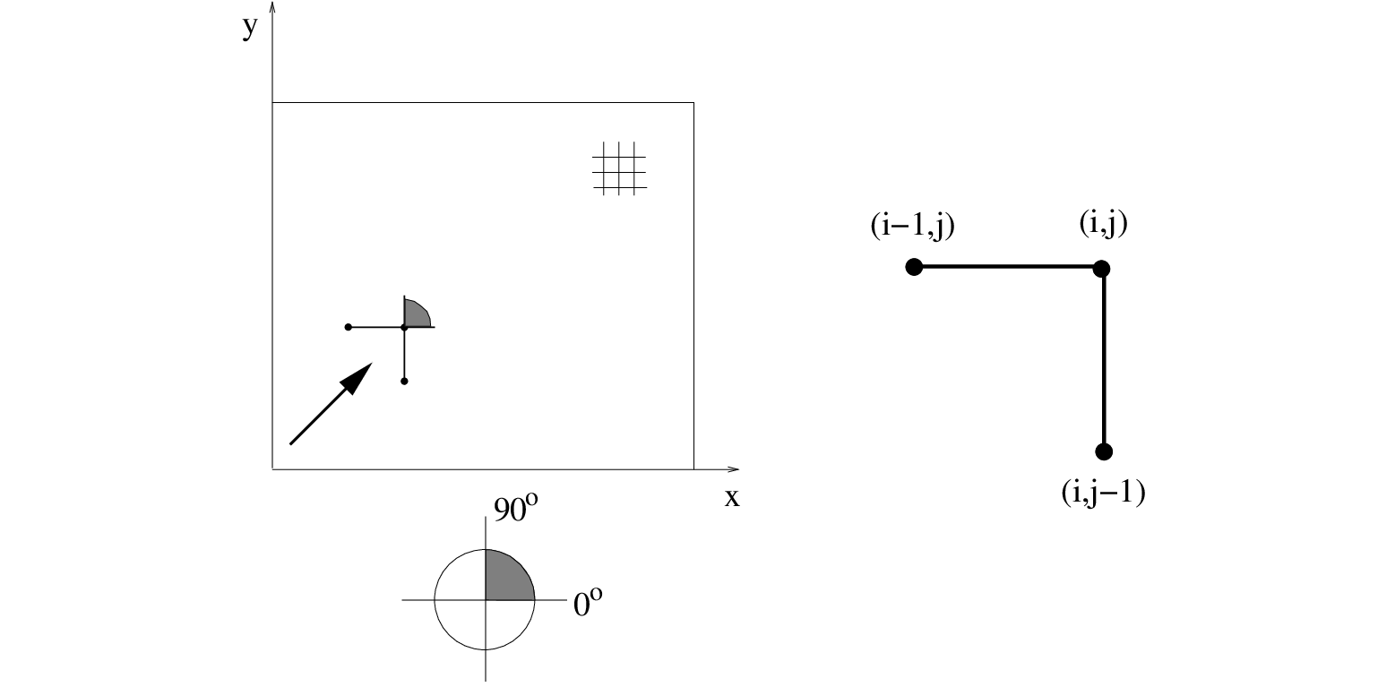
and  positive during the first sweep, see Figure 3.4,
 |
 (3.57)
 is the time step, and
  and
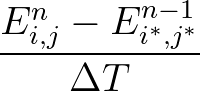
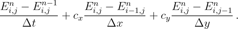
and  are the mesh spaces. This approximation can be viewed as the well-known semi-Lagrangian approximation, which is rewritten as
 (3.58)
 (3.60)
 and
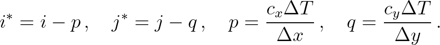
and  are the Courant numbers. They are not integers, and therefore
  is not a grid point. This point, however, lies on the wave characteristic. The quantity
 can be
interpreted as the value of
can be
interpreted as the value of  at time
  in which is being convected in
  in a lapsed time
  .
This value is simply obtained from the interpolation of the surrounding values
.
This value is simply obtained from the interpolation of the surrounding values  ,
,
 ,
,  and
and  in the
  plane. In this case, there is no restriction on time step as the characteristic lies inside the computational stencil.
Note that the lapsed time is a function of time step and grid sizes
and , and is called the Lagrangian time step, which should not be confused with the Eulerian time step . Generally,
plane. In this case, there is no restriction on time step as the characteristic lies inside the computational stencil.
Note that the lapsed time is a function of time step and grid sizes
and , and is called the Lagrangian time step, which should not be confused with the Eulerian time step . Generally,
 .
.
 (3.61)
.
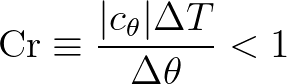
Thus, for physical consistency, a restriction on the time step must be imposed in order for the wave directions not to cross each other and the boundaries of a quadrant in the spectral space.
Specifically, the Courant number based on and
(3.61)
.
Thus, for physical consistency, a restriction on the time step must be imposed in order for the wave directions not to cross each other and the boundaries of a quadrant in the spectral space.
Specifically, the Courant number based on and  (i.e. directional bin) must be less than unity, that is,
 the turning rate3.7.
This condition is a sufficient one and implies the Lipschitz criterion.
the turning rate3.7.
This condition is a sufficient one and implies the Lipschitz criterion.
 ,
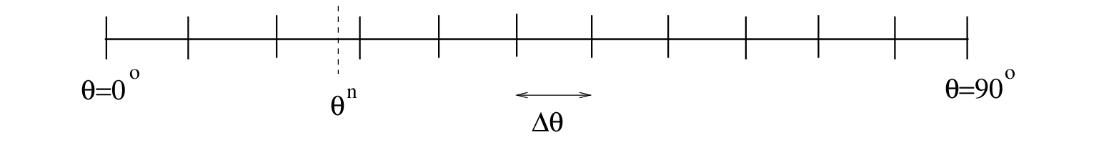
see Figure 3.4).
For example, consider the first sweep, see Figure 3.4, the boundaries of the first quadrant are the lines 0 and 90. Next, we consider the directional
sector in the spectral space associated with the considered sweep, see Figure 3.5.
We shall show that condition, Eq. (3.62), is sufficient to assure that 1) during the distance travelled in
,
see Figure 3.4).
For example, consider the first sweep, see Figure 3.4, the boundaries of the first quadrant are the lines 0 and 90. Next, we consider the directional
sector in the spectral space associated with the considered sweep, see Figure 3.5.
We shall show that condition, Eq. (3.62), is sufficient to assure that 1) during the distance travelled in  direction is at most
and 2) wave energy propagating in any bin in direction will not cross the boundaries of the directional sector,
except for the first and last bins. Hence, this prevents wave rays from intersecting each other.
Note that we implicitly assume that the net change in mean wave direction within the distance covered during is less than the directional resolution.
Since, by definition,
direction is at most
and 2) wave energy propagating in any bin in direction will not cross the boundaries of the directional sector,
except for the first and last bins. Hence, this prevents wave rays from intersecting each other.
Note that we implicitly assume that the net change in mean wave direction within the distance covered during is less than the directional resolution.
Since, by definition,
 (3.63)
 , we choose an arbitrary point,
  , inside the directional sector; see Figure 3.5.
If
, inside the directional sector; see Figure 3.5.
If
 then, Eqs. (3.64) and (3.62) imply
 , and hence the chosen point at next time step,
  , still lies inside the directional sector. If
 , i.e. in the first bin, then one obtains
![$\displaystyle \theta^n = \theta^{n-1} + \frac{\Delta T}{\Delta \theta} \left[ (...
...1}) c_\theta(\theta=0^o) + \theta^{n-1} c_\theta(\theta=\Delta \theta) \right]
$](img1085.png) (3.65)
(3.65)
 (3.66)
 and
and
 then, the point at next step will be keep inside the directional sector, if Eq. (3.62) holds. In other cases the energy is leaving
through boundary
then, the point at next step will be keep inside the directional sector, if Eq. (3.62) holds. In other cases the energy is leaving
through boundary  , though the change in direction is limited to the adjacent directional bin of the other quadrant.
This holds also for the last bin and the corresponding right boundary
, though the change in direction is limited to the adjacent directional bin of the other quadrant.
This holds also for the last bin and the corresponding right boundary  .
.
 space, propagating at an angle with the positive
  axis.
There is a bottom gradient along this axis so that refraction is present. There are no currents.
The associated characteristic or wave ray is given by
axis.
There is a bottom gradient along this axis so that refraction is present. There are no currents.
The associated characteristic or wave ray is given by
 . This is the
spatial turning rate, i.e. the change in wave direction per unit forward distance.
Hence, the directional turn of the wave crest over a distance is given by
. This is the
spatial turning rate, i.e. the change in wave direction per unit forward distance.
Hence, the directional turn of the wave crest over a distance is given by
 (3.67)
 (3.68)
 is the wave number,
  is the frequency,
  is the water depth and
  is the coordinate along the wave crest (i.e. orthogonal to the propagation direction). On a coarse grid,
the depth difference in two adjacent grid points
is the coordinate along the wave crest (i.e. orthogonal to the propagation direction). On a coarse grid,
the depth difference in two adjacent grid points  , and thereby , can be very large, especially for low-frequency components in very shallow water
(see also Section 3.8.5).
This implies that the Lipschitz condition may be violated, i.e.
, and thereby , can be very large, especially for low-frequency components in very shallow water
(see also Section 3.8.5).
This implies that the Lipschitz condition may be violated, i.e.
 .
in the shallowest grid point can be simply too large due to a large difference in bottom levels over one mesh width,
so that wave energy will change direction over more than some directional bins
or even the directional sector, so that wave rays falsely intersect each other.
To prevent this artefact a limitation on seems to be justified. Recalling Eq. (3.62), a limitation would be
.
in the shallowest grid point can be simply too large due to a large difference in bottom levels over one mesh width,
so that wave energy will change direction over more than some directional bins
or even the directional sector, so that wave rays falsely intersect each other.
To prevent this artefact a limitation on seems to be justified. Recalling Eq. (3.62), a limitation would be
 (3.70)
as a fraction of
(3.70)
as a fraction of
 (3.71)
 (3.72)
 a user-defined maximum Courant number, which is generally smaller than 1. (In SWAN, the default value is
 .)
Often the desired time step is such that the first term between brackets can be safely neglected. This implies a slightly more restriction
on the turning rate and, in turn, a safety margin in the CFL condition, as follows
.
In fact, we need to find a good estimate for which solely depends on .
However, it is unlikely that this measure affects the solution nearshore or on fine grids, since the turning rate will not too much vary over one (spatial) step.
This is an effective survival measure in the sense that it prevents the excessive refraction without deteriorating the solution
elsewhere.
.)
Often the desired time step is such that the first term between brackets can be safely neglected. This implies a slightly more restriction
on the turning rate and, in turn, a safety margin in the CFL condition, as follows
.
In fact, we need to find a good estimate for which solely depends on .
However, it is unlikely that this measure affects the solution nearshore or on fine grids, since the turning rate will not too much vary over one (spatial) step.
This is an effective survival measure in the sense that it prevents the excessive refraction without deteriorating the solution
elsewhere.
The SWAN team 2026-03-13