Next: The problem with refraction Up: On the approximation of Previous: Introduction
In this section we focus on the following transport processes: shoaling and refraction. Calculating the wave shoaling and refraction
effects is necessary to predict accurately shallow water wave conditions, either in the surf zone, across the main channels in estuaries, or
across the seamounts. Throughout this section we assume the absence of the non-conservative source/sink terms, such as wind input, nonlinear wave-wave interactions
and energy dissipation.
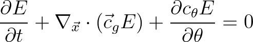
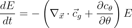
The governing equation is the following wave energy balance (ambient current is not included)
 space are generally not straight lines due
to a varying seabed topography.
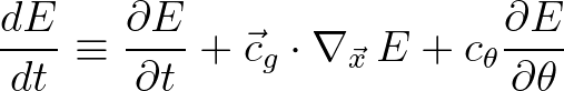
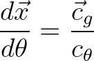
Along the characteristics the wave energy fluxes
space are generally not straight lines due
to a varying seabed topography.
Along the characteristics the wave energy fluxes  and
and  are constant
(Whitham, 1974).
are constant
(Whitham, 1974).
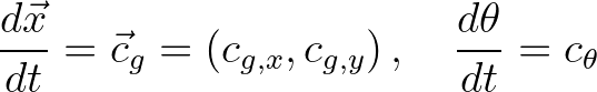
 defined as
space is in this case the direction of propagation
(with group velocity). By virtue of Eq. (3.47), the total energy is thus constant along the
same characteristic. However, due to depth variations, wave energy will either increase or decrease along its
curved characteristic.
defined as
space is in this case the direction of propagation
(with group velocity). By virtue of Eq. (3.47), the total energy is thus constant along the
same characteristic. However, due to depth variations, wave energy will either increase or decrease along its
curved characteristic.
 ,
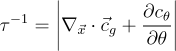
which is the typical time scale for wave energy transport to reach steady state after being disturbed.
It is given by
,
which is the typical time scale for wave energy transport to reach steady state after being disturbed.
It is given by
 (3.51)
 .
Causality requires that wave energy propagates in the right direction along its characteristic, and at the right speed.
For example, causality problem can be present in an implicit scheme that propagates wave energy across a large distance using a large time step.
In other words, if this time step is too large, some wave components getting ahead of themselves and leaving behind some other components ahead.
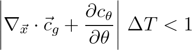
To prevent this, temporal, spatial and directional changes in the numerical and exact solutions must go hand in hand.
This implies that
.
Causality requires that wave energy propagates in the right direction along its characteristic, and at the right speed.
For example, causality problem can be present in an implicit scheme that propagates wave energy across a large distance using a large time step.
In other words, if this time step is too large, some wave components getting ahead of themselves and leaving behind some other components ahead.
To prevent this, temporal, spatial and directional changes in the numerical and exact solutions must go hand in hand.
This implies that
 . Hence, a sufficient condition for accurate
integration reads
. Hence, a sufficient condition for accurate
integration reads
 (3.53)
 the length of the wave number vector (cf. Eq. (2.14)).
This criterion implies that at locations with relatively large bottom slopes, the step size must reduce
locally to prevent inaccuracies. This step size is determined by the temporal, spatial and directional resolutions.
In this regard, the interpretation of the Lipschitz criterion (3.52) is that the maximum step size
is determined by the numerical accuracy rather than by the numerical stability.
This accuracy aspect is related to the curvature of the wave propagation field (due to change in wave direction over a certain distance)
at the grid and time resolutions applied.
the length of the wave number vector (cf. Eq. (2.14)).
This criterion implies that at locations with relatively large bottom slopes, the step size must reduce
locally to prevent inaccuracies. This step size is determined by the temporal, spatial and directional resolutions.
In this regard, the interpretation of the Lipschitz criterion (3.52) is that the maximum step size
is determined by the numerical accuracy rather than by the numerical stability.
This accuracy aspect is related to the curvature of the wave propagation field (due to change in wave direction over a certain distance)
at the grid and time resolutions applied.
 50 m is not uncommon in
SWAN applications.
An important assumption made in this consideration is that the transport velocities
50 m is not uncommon in
SWAN applications.
An important assumption made in this consideration is that the transport velocities  and
and  do not much vary over a grid size,
so that Lipschitz criterion (3.52) is most likely met.
This is reasonable as the wave characteristics are more or less non-curved lines (during the elapsed time step),
because the propagation in the
space is slowly time varying.
This is generally true in coastal applications.
50 km. However, there are exceptions. An
example are the seamounts in the deeper parts of the open ocean. At such locations, the depth may
vary from one grid point to the next by a factor of 10 or so or even more. In such a case, the value of the turning rate at the
shallowest grid point is not representative anymore with respect to the distance between the two
considered grid points. Hence, criterion (3.52) is violated, and computed spectral wave components will simply turn too
much and jump multiple directional bins in one distance step. The result is that a number of wave components in one sweep within one distance step overtakes
some other bins in another sweep ahead, which implies that causality is violated, resulting in a possible model instability.
To circumvent this we must refine the computational grid locally to resolve the local bathymetric features, and the Lipschitz criterion
(3.52) can be helpful in this. The consequences will be discussed in the following section.
do not much vary over a grid size,
so that Lipschitz criterion (3.52) is most likely met.
This is reasonable as the wave characteristics are more or less non-curved lines (during the elapsed time step),
because the propagation in the
space is slowly time varying.
This is generally true in coastal applications.
50 km. However, there are exceptions. An
example are the seamounts in the deeper parts of the open ocean. At such locations, the depth may
vary from one grid point to the next by a factor of 10 or so or even more. In such a case, the value of the turning rate at the
shallowest grid point is not representative anymore with respect to the distance between the two
considered grid points. Hence, criterion (3.52) is violated, and computed spectral wave components will simply turn too
much and jump multiple directional bins in one distance step. The result is that a number of wave components in one sweep within one distance step overtakes
some other bins in another sweep ahead, which implies that causality is violated, resulting in a possible model instability.
To circumvent this we must refine the computational grid locally to resolve the local bathymetric features, and the Lipschitz criterion
(3.52) can be helpful in this. The consequences will be discussed in the following section.
The SWAN team 2026-03-13