Next: The sweeping algorithm Up: Numerical method Previous: Numerical method
For the sake of clarity of the algorithm description below, we put all the terms but the time derivative and propagation term in the geographical space of Eq. (2.16)
in one term
 :
:
 the geographic velocity vector.
 is stored at the vertices and Eq. (8.5) is solved in each vertex.
We note that the values at boundary vertices are fixed during the computation.
is stored at the vertices and Eq. (8.5) is solved in each vertex.
We note that the values at boundary vertices are fixed during the computation.
 is the time step and
  is the time step counter. The main property of this approximation is that it does not suffer from the stability restriction
imposed by the CFL condition inherent in the explicit methods as employed in most spectral models. In principle, the time step is limited only by
the desired temporal accuracy. This procedure, however, involves the solution of a large system of equations.
is the time step counter. The main property of this approximation is that it does not suffer from the stability restriction
imposed by the CFL condition inherent in the explicit methods as employed in most spectral models. In principle, the time step is limited only by
the desired temporal accuracy. This procedure, however, involves the solution of a large system of equations.
 |
 |
 = (
= ( ,
, ) to the
Cartesian one
) to the
Cartesian one  = (
= ( ,
, ).
Based on this transformation
).
Based on this transformation
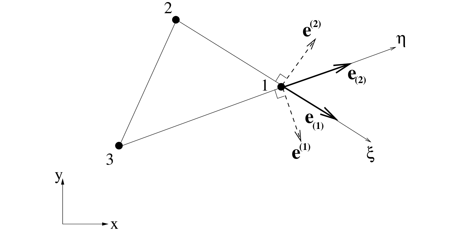
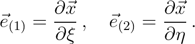
 , we have the following base vectors that are tangential to the coordinate lines and , respectively,
 (8.7)
(8.7)
 (8.8)
and , respectively (see Figure 8.3). Moreover, they are reciprocal to the base vectors, i.e.
(8.8)
and , respectively (see Figure 8.3). Moreover, they are reciprocal to the base vectors, i.e.
 (8.9)
(8.9)
 is Kronecker delta (which is unity if
  =
=  , and zero otherwise). Using Cramer's rule, one can find
Next, we expand the propagation term of Eq. (8.6):
![$\displaystyle \nabla_{\vec{x}} \cdot [\vec{c}_{\vec{x}} N] = \frac{\partial c_x N}{\partial x} + \frac{\partial c_y N}{\partial y} \, ,
$](img1426.png) (8.11)
(8.11)
 and
and  are the
  and
and  components of the wave propagation vector
 , respectively.
Using the chain rule, we obtain
, respectively.
Using the chain rule, we obtain
 ,
,  and
and  , respectively.
Here, we choose the mapping
such that
, respectively.
Here, we choose the mapping
such that  =
=  = 1.
The approximation is completed by substituting (8.13) in (8.12):
= 1.
The approximation is completed by substituting (8.13) in (8.12):
 and
and
 in Eq. (8.14) are given by Eqs. (8.10), while
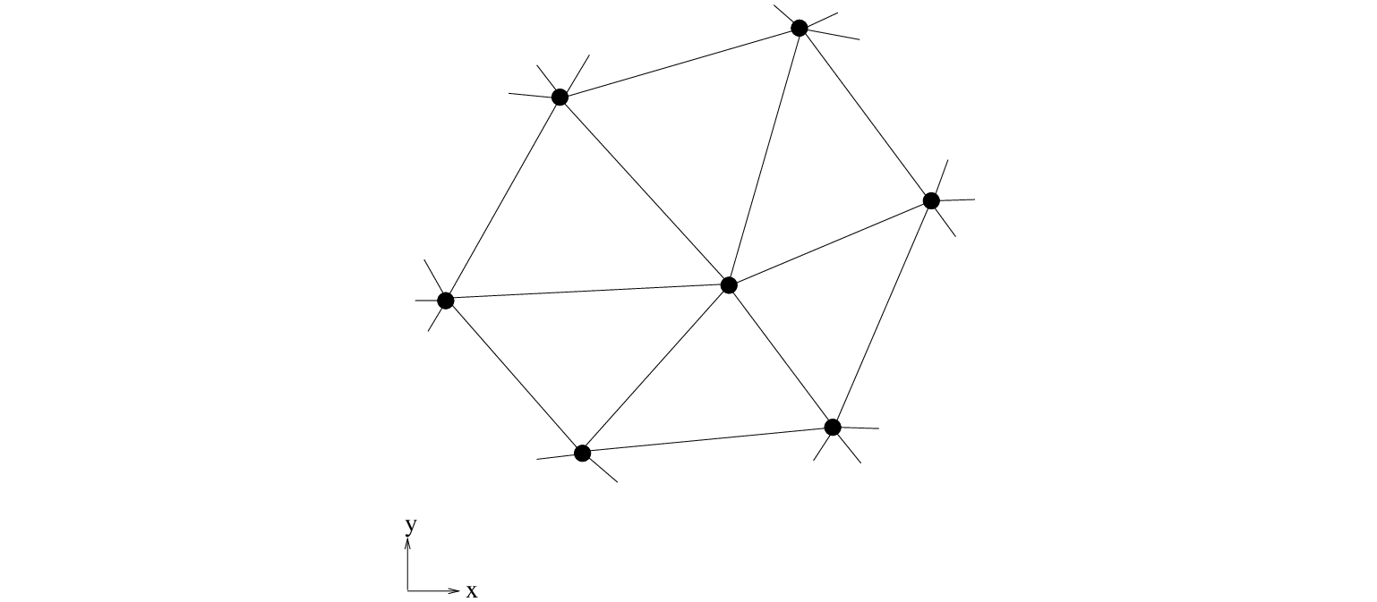
the base vectors are calculated according to
in Eq. (8.14) are given by Eqs. (8.10), while
the base vectors are calculated according to
 the position vector of vertex
  in a Cartesian coordinate system.
This space discretization is of lowest order accurate and conserves action (see Section 8.7).
in a Cartesian coordinate system.
This space discretization is of lowest order accurate and conserves action (see Section 8.7).
 everywhere.
This finite difference BSBT scheme appears to be identical to the well-known N(arrow) scheme, based on the fluctuation splitting method,
on regular, triangular grids obtained from triangulation of rectangles with diagonals aligning with the wave characteristic as much as possible
(see Struijs, 1994, pp. 63-64).
Hence, the BSBT scheme share with the N scheme in many respects: it is multidimensional, first order accurate, optimal in terms of cross-diffusion, monotone, conservative,
narrow stencil and consistent with local wave characteristics (see Section 3.2.1), but they are not identical in general.
everywhere.
This finite difference BSBT scheme appears to be identical to the well-known N(arrow) scheme, based on the fluctuation splitting method,
on regular, triangular grids obtained from triangulation of rectangles with diagonals aligning with the wave characteristic as much as possible
(see Struijs, 1994, pp. 63-64).
Hence, the BSBT scheme share with the N scheme in many respects: it is multidimensional, first order accurate, optimal in terms of cross-diffusion, monotone, conservative,
narrow stencil and consistent with local wave characteristics (see Section 3.2.1), but they are not identical in general.
 and
and  at vertices 2 and 3 of triangle
  123,
the wave action in vertex 1 is readily determined according to
123,
the wave action in vertex 1 is readily determined according to
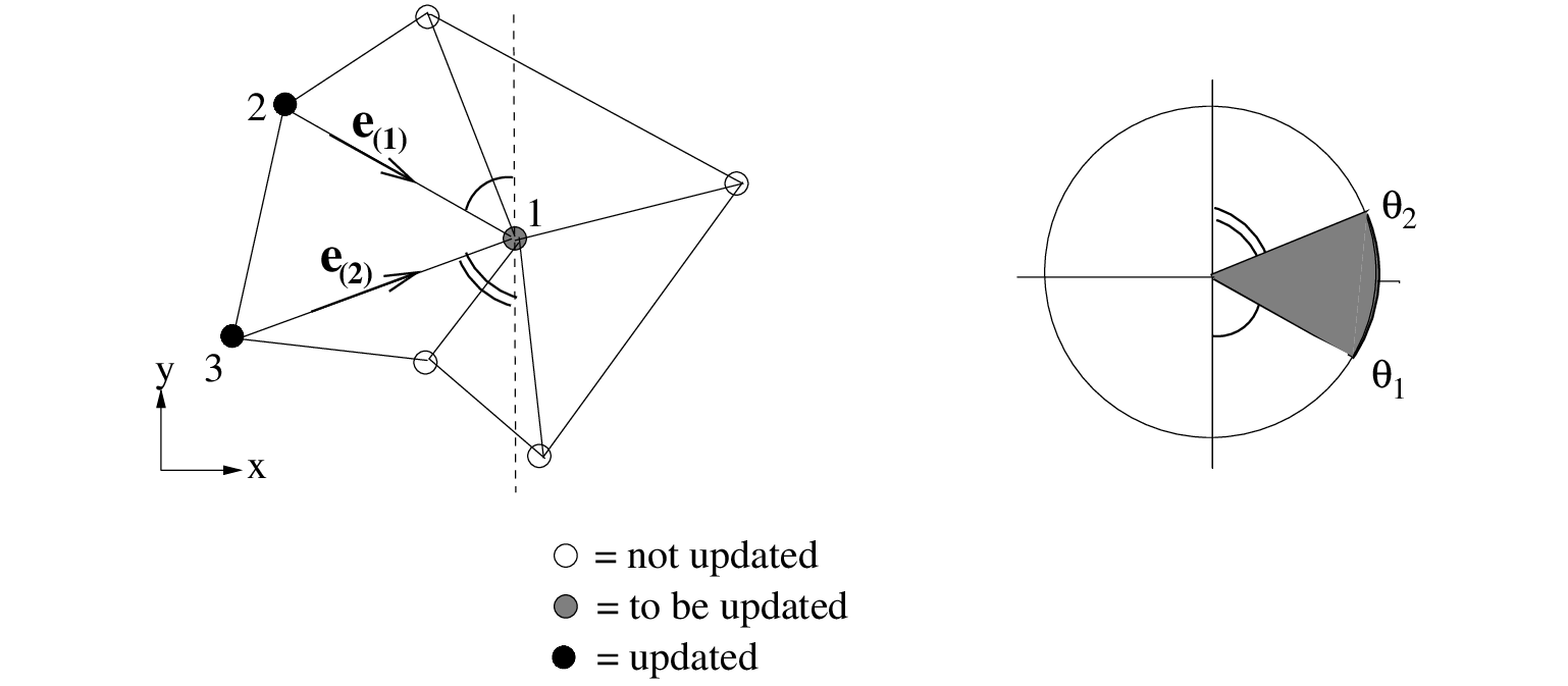
The wave directions between faces  and
and  enclose all wave energy propagation in between the corresponding directions
  and
and  as
indicated as a shaded sector in Figure 8.2.
This sector is the domain of dependence of Eq. (8.16) in vertex 1.
Since, the wave characteristics lie within this directional sector, this ensures that the CFL number
used will properly capture the propagation of wave action towards vertex 1. So, propagation is in line with the causality principle and is not subjected to a CFL stability criterion.
Next, the term
as
indicated as a shaded sector in Figure 8.2.
This sector is the domain of dependence of Eq. (8.16) in vertex 1.
Since, the wave characteristics lie within this directional sector, this ensures that the CFL number
used will properly capture the propagation of wave action towards vertex 1. So, propagation is in line with the causality principle and is not subjected to a CFL stability criterion.
Next, the term  in Eq. (8.16) is discretized implicitly in the sector considered.
Since the approximation in the spectral space and the linearization of the source terms are well explained in Section 3.3, we shall not pursue them any further.
Eq. (8.16) constitute a coupled set of linear, algebraic equations for all spectral bins within the sector considered at vertex 1. The solution is found by means
of an iterative solver; see Section 3.3 for details.
in Eq. (8.16) is discretized implicitly in the sector considered.
Since the approximation in the spectral space and the linearization of the source terms are well explained in Section 3.3, we shall not pursue them any further.
Eq. (8.16) constitute a coupled set of linear, algebraic equations for all spectral bins within the sector considered at vertex 1. The solution is found by means
of an iterative solver; see Section 3.3 for details.
The update of vertex 1 is completed when all surrounding cells have been treated. This allows waves to transmit from all directions.
Due to refraction and nonlinear interactions, wave energy shifts in the spectral space from one directional sector to another. This is taken into account properly
by repeating the whole procedure with
converging results.
The SWAN team 2026-03-13
![$\displaystyle \frac{\partial N}{\partial t} + \nabla_{\vec{x}} \cdot [\vec{c}_{\vec{x}} N] = F
$](img1414.png)
![$\displaystyle \frac{N^n - N^{n-1}}{\Delta t} + \nabla_{\vec{x}} \cdot [\vec{c}_{\vec{x}} N^n] = F^n
$](img1417.png)

![$\displaystyle \nabla_{\vec{x}} \cdot [\vec{c}_{\vec{x}} N] = e^{(1)}_1 \frac{\p...
...ial c_y N}{\partial \xi} + e^{(2)}_2 \frac{\partial c_y N}{\partial \eta} \, .
$](img1428.png)

![$\displaystyle \nabla_{\vec{x}} \cdot [\vec{c}_{\vec{x}} N] \approx c_x N\vert _...
...rt _3^1 e^{(2)}_1 + c_y N\vert _2^1 e^{(1)}_2 + c_y N\vert _3^1 e^{(2)}_2 \, .
$](img1435.png)

![$\displaystyle \left[ \frac{1}{\Delta t} + c_{x,1} \left( e^{(1)}_1 + e^{(2)}_1 \right) + c_{y,1} \left( e^{(1)}_2 + e^{(2)}_2 \right) \right] N_1^n =$](img1443.png)
