Next: Governing equations in curvilinear Up: Numerical approaches Previous: The problem with refraction
One observes that the phase-space equation (2.225) (2.230) is formulated in
 space, whereas SWAN operates in frequency-direction space.
In particular due to the QC scattering term that involves a Fourier transform from physical space to a wave number space, one should stick to the
space, whereas SWAN operates in frequency-direction space.
In particular due to the QC scattering term that involves a Fourier transform from physical space to a wave number space, one should stick to the  space in solving the governing equation
for the statistics of the wave field (as represented by the Wigner distribution). Examples of such an approach are presented in Smit et al. (2015a) and Akrish et al. (2020).
space in solving the governing equation
for the statistics of the wave field (as represented by the Wigner distribution). Examples of such an approach are presented in Smit et al. (2015a) and Akrish et al. (2020).
Here, we take a different route by applying a transformation to
 space.
We first define the Wigner distribution in the frequency-direction space and subsequently
transform it to the space. Next, we compute
the scattering term in the phase space using the transformed Wigner spectrum, and lastly, the result is transformed back to the frequency-direction space.
space.
We first define the Wigner distribution in the frequency-direction space and subsequently
transform it to the space. Next, we compute
the scattering term in the phase space using the transformed Wigner spectrum, and lastly, the result is transformed back to the frequency-direction space.
For the purpose of the implementation in SWAN we thus consider the following equation
 the Wigner distribution in the appropriate spectral space and
 the Jacobian.
Note that for evaluating the source term
the Jacobian.
Note that for evaluating the source term
 we thus priorly need to compute
 .
.
 by means of the introduction of the cross correlations.
It basically implies conservation in the presence of ambient current.
So for computing the spectral moments and, in turn, the integral parameters (e.g. significant wave height and mean period) one must consider the
product
by means of the introduction of the cross correlations.
It basically implies conservation in the presence of ambient current.
So for computing the spectral moments and, in turn, the integral parameters (e.g. significant wave height and mean period) one must consider the
product  with which the integration over spectral space can be performed. Additionally, recall that
  can take on negative values.
This implies, for example, that the conservative elimination approach as outlined in Section 3.2.4 should not be applied because otherwise the moments will be wrongly computed.
Note that by definition,
can take on negative values.
This implies, for example, that the conservative elimination approach as outlined in Section 3.2.4 should not be applied because otherwise the moments will be wrongly computed.
Note that by definition,
 .
space to
space, and vice versa.
For instance, two interacting waves
.
space to
space, and vice versa.
For instance, two interacting waves  and
and  having the same frequency
 create a cross contribution at
frequency
create a cross contribution at
frequency
 , with the result that a mapping error occur when one is transforming
  to
to
 .
Although the cross correlations may thus be aliased at offset frequencies, we expect that such aliasing errors would prove to be small enough to be accepted (see also Appendix C of Smit et al., 2015b).
.
Although the cross correlations may thus be aliased at offset frequencies, we expect that such aliasing errors would prove to be small enough to be accepted (see also Appendix C of Smit et al., 2015b).
 .
As a result, the modelling of these wave processes do not appear explicitly as conventional transport terms in Eq. (3.86) (viz. the third and fourth terms of Eq. (2.16)).
There are two reasons for this approach. First, it circumvents the stiffness of the equation that otherwise would occur owing to the relatively rapid variations in the medium,
thus leading to unnecessary and excessive resolution in the spectral space (Akrish et al., 2020).
Second, by means of the local plane approximation of Smit et al. (2015a) the refraction term
.
As a result, the modelling of these wave processes do not appear explicitly as conventional transport terms in Eq. (3.86) (viz. the third and fourth terms of Eq. (2.16)).
There are two reasons for this approach. First, it circumvents the stiffness of the equation that otherwise would occur owing to the relatively rapid variations in the medium,
thus leading to unnecessary and excessive resolution in the spectral space (Akrish et al., 2020).
Second, by means of the local plane approximation of Smit et al. (2015a) the refraction term
 could have been extracted out of the integral
in Eq. (2.230), which is, however, formulated in space rather than in
space.
This would mean an additional error-prone coordinate mapping through the Jacobian transformation (and interpolation).
,
could have been extracted out of the integral
in Eq. (2.230), which is, however, formulated in space rather than in
space.
This would mean an additional error-prone coordinate mapping through the Jacobian transformation (and interpolation).
,
 and
and  spaces, respectively, and after this we provide an outline of the QC implementation.
space in which the effects of wave interference are resolved.
The origin and the size of its wave number domain
spaces, respectively, and after this we provide an outline of the QC implementation.
space in which the effects of wave interference are resolved.
The origin and the size of its wave number domain
 is
determined by the transformation of the user-defined spectral
domain (commonly defined as a directional sector).
Apart from this, the determination of the wave number grid spacing is a crucial factor as explained in the following.
is
determined by the transformation of the user-defined spectral
domain (commonly defined as a directional sector).
Apart from this, the determination of the wave number grid spacing is a crucial factor as explained in the following.
 . The grid size as denoted by
  is then set to this standard deviation.
In relation to this, the coherent length scale of the correlated wave field is defined as
is then set to this standard deviation.
In relation to this, the coherent length scale of the correlated wave field is defined as
 (Smit et al., 2015a).
Note that the two-dimensional
(Smit et al., 2015a).
Note that the two-dimensional  grid thus obtained is equidistant in both directions.
 to obtain
 .
To this end, the so-called coherent region in
space is defined as a square
with the origin in the center and, owing to its compact support, its side length is half the correlation length, thus
.
To this end, the so-called coherent region in
space is defined as a square
with the origin in the center and, owing to its compact support, its side length is half the correlation length, thus
 .
Furthermore, this domain is equipped with a grid consisting of
.
Furthermore, this domain is equipped with a grid consisting of
 equally spaced points separated by a distance
 in each direction.
The specification of
in each direction.
The specification of  will be discussed below.
 over which the integral of Eq. (2.230) is to be performed. This domain is conjugated to
 and,
since the Nyquist wave length is
and,
since the Nyquist wave length is
 , it is truncated to
 with
with
 .
This maximum scattering wave number can be set directly by the
user or, alternatively, prescribed as a multiple of the peak (or mean) wave number at the wavemaker
.
This maximum scattering wave number can be set directly by the
user or, alternatively, prescribed as a multiple of the peak (or mean) wave number at the wavemaker  ,
,
 with
with  usually 0.5, 1 or 2.
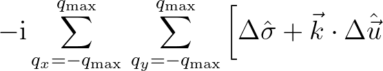
is subsequently discretized into uniform grid of
usually 0.5, 1 or 2.
is subsequently discretized into uniform grid of  bins with grid size
  . We select
 so as
to avoid interpolation errors in computing the convolution integral of Eq. (2.230). Consequently,
so as
to avoid interpolation errors in computing the convolution integral of Eq. (2.230). Consequently,
 .
From the above we have that
.
From the above we have that
 . So, there is a one-to-one mapping between
the grid of
and the grid of , thus requiring no interpolation.
. So, there is a one-to-one mapping between
the grid of
and the grid of , thus requiring no interpolation.
 ,
,
 and
and
 the discrete Fourier transform of, respectively,
![$\displaystyle \Delta \sigma = {\cal W}(x^\prime)\,{\cal W}(y^\prime) \left [ \,\sigma(x+x^\prime,y+y^\prime,k_x,k_y) - \sigma(x,y,k_x,k_y) \,\right ]$](img1170.png) | ||||
![$\displaystyle \Delta c_g = {\cal W}(x^\prime)\,{\cal W}(y^\prime) \left [ \,c_g(x+x^\prime,y+y^\prime,k_x,k_y) - c_g(x,y,k_x,k_y) \,\right ]$](img1171.png) | ||||
![$\displaystyle \Delta \vec{u} = {\cal W}(x^\prime)\,{\cal W}(y^\prime) \left [ \,\vec{u}(x+x^\prime,y+y^\prime) - \vec{u}(x,y) \,\right ]$](img1172.png) |
 is a window function which tapers the function to be transformed near the
boundaries of the
is a window function which tapers the function to be transformed near the
boundaries of the  interval (and so to reduce or possibly remove any jump discontinuity of the outcome). A standard Tukey window is utilized and is given by
![$\displaystyle {\cal W}(z) =
\left\{
\begin{array}{ll}
\frac{1}{2}\left\{ 1 +...
...ight ]\right ) \right\}, & (1-\gamma)\,\ell < z \leq \ell
\end{array} \right.
$](img1175.png) (3.88)
(3.88)
 the side of the square coherent zone centered at
  and
and
 a dimensionless taper parameter. In SWAN, it is set hardcoded to
  .
.
 is discretized by means of second order central differences
on structured grids.
In case of an unstructured mesh, the Green-Gauss theorem with the assumption of a constant gradient over the centroid dual volume is then applied; viz. Eq. (8.35).
is discretized by means of second order central differences
on structured grids.
In case of an unstructured mesh, the Green-Gauss theorem with the assumption of a constant gradient over the centroid dual volume is then applied; viz. Eq. (8.35).
![$\displaystyle \frac{\partial W}{\partial t} + \nabla_{\vec{x}} \cdot [({\vec{c}}_g + \vec{u}) W] = J^{-1}\,S_{\rm qc}
$](img1131.png)
![$\displaystyle \biggl. -\frac{{\rm i}}{2}\Bigl( \Delta {\hat{c_g}}\, \frac{\vec{...
...bla_{\vec{x}} \biggr]\,
W(x,y,k_x-\frac{q_x}{2},k_y-\frac{q_y}{2}) + \rm {c.c.}$](img1166.png)